
Step 8: Slip on Two Faults and Power-law Viscoelastic Materials#
Features
Triangular cells
pylith.meshio.MeshIOPetsc
pylith.problems.TimeDependent
pylith.bc.DirichletTimeDependent
spatialdata.spatialdb.SimpleDB
spatialdata.spatialdb.ZeroDB
pylith.meshio.OutputSolnBoundary
pylith.meshio.DataWriterHDF5
Quasi-static simulation
pylith.materials.Elasticity
pylith.materials.IsotropicPowerLaw
pylith.faults.FaultCohesiveKin
pylith.faults.KinSrcStep
spatialdata.spatialdb.UniformDB
spatialdata.spatialdb.CompositeDB
Simulation parameters#
In this example we replace the linear, isotropic Maxwell viscoelastic bulk rheology in the slab in Step 7 with an isotropic powerlaw viscoelastic rheology.
The other parameters remain the same as those in Step 6.
The parameters specific to this example are in step08_twofaults_powerlaw.cfg.
[pylithapp.problem.materials]
slab.bulk_rheology = pylith.materials.IsotropicPowerLaw

[pylithapp.problem.materials.slab]
db_auxiliary_field = spatialdata.spatialdb.CompositeDB
db_auxiliary_field.description = Power law material properties

bulk_rheology.auxiliary_subfields.power_law_reference_strain_rate.basis_order = 0
bulk_rheology.auxiliary_subfields.power_law_reference_stress.basis_order = 0
bulk_rheology.auxiliary_subfields.power_law_exponent.basis_order = 0

[pylithapp.problem.materials.slab.db_auxiliary_field]
# Elastic properties
values_A = [density, vs, vp]
db_A = spatialdata.spatialdb.SimpleDB
db_A.description = Elastic properties for slab
db_A.iohandler.filename = mat_elastic.spatialdb

# Power law properties
values_B = [
	 power_law_reference_stress,  power_law_reference_strain_rate,  power_law_exponent,
	 viscous_strain_xx, viscous_strain_yy, viscous_strain_zz, viscous_strain_xy,
	 reference_stress_xx, reference_stress_yy, reference_stress_zz, reference_stress_xy,
	 reference_strain_xx, reference_strain_yy, reference_strain_zz, reference_strain_xy,
	 deviatoric_stress_xx,  deviatoric_stress_yy,  deviatoric_stress_zz,  deviatoric_stress_xy
	 ]
db_B = spatialdata.spatialdb.SimpleDB
db_B.description = Material properties specific to power law bulk rheology for the slab
db_B.iohandler.filename = mat_powerlaw.spatialdb
db_B.query_type = linear
Power-law spatial database#
New in v4.0.0
We use the utility script pylith_powerlaw_gendb (see pylith_powerlaw_gendb) to generate the spatial database mat_powerlaw.spatialdb with the power-law bulk rheology parameters.
We provide the parameters for pylith_powerlaw_gendb in powerlaw_gendb.cfg, which follows the same formatting conventions as the PyLith parameter files.
pylith_powerlaw_gendb powerlaw_gendb.cfg
Running the simulation#
$ pylith step08_twofaults_powerlaw.cfg

# The output should look something like the following.
 >> /software/unix/py3.12-venv/pylith-debug/lib/python3.12/site-packages/pylith/apps/PyLithApp.py:77:main
 -- pylithapp(info)
 -- Running on 1 process(es).
 >> /software/unix/py3.12-venv/pylith-debug/lib/python3.12/site-packages/pylith/meshio/MeshIOObj.py:38:read
 -- meshiopetsc(info)
 -- Reading finite-element mesh
 >> /src/cig/pylith/libsrc/pylith/meshio/MeshIO.cc:85:void pylith::meshio::MeshIO::read(pylith::topology::Mesh *, const bool)
 -- meshiopetsc(info)
 -- Component 'reader': Domain bounding box:
    (-100000, 100000)
    (-100000, 0)

# -- many lines omitted --

25 TS dt 0.2 time 4.8
    0 SNES Function norm 2.142894303456e-06
    Linear solve converged due to CONVERGED_ATOL iterations 22
    1 SNES Function norm 6.320440892495e-09
    Linear solve converged due to CONVERGED_ATOL iterations 14
    2 SNES Function norm 1.048804327259e-10
  Nonlinear solve converged due to CONVERGED_FNORM_ABS iterations 2
26 TS dt 0.2 time 5.
 >> /software/unix/py3.12-venv/pylith-debug/lib/python3.12/site-packages/pylith/problems/Problem.py:199:finalize
 -- timedependent(info)
 -- Finalizing problem.
As in Step 7, the simulation advances 26 time steps. With a nonlinear bulk rheology, the nonlinear solver now requires a few iterations to converge at each time step.
Visualizing the results#
In Fig. 109 we use the pylith_viz utility to visualize the x displacement field.
You can move the slider or use the p and n keys to change the increment or decrement time.
pylith_viz --filename=output/step08_twofaults_powerlaw-domain.h5 warp_grid --component=x
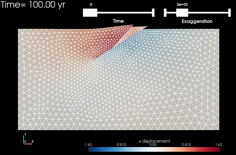
Fig. 109 Solution for Step 8 at t=100 years. The colors of the shaded surface indicate the x displacement, and the deformation is exaggerated by a factor of 1000. The undeformed configuration is shown by the gray wireframe. Our parameters for the power-law bulk rheology result in much less viscoelastic relaxation in this case compared to Step 7.#