
Step 5: Static Coseismic Slip#
This example involves a static simulation that solves for the deformation from prescribed coseismic slip on the main fault. We specify 2 meters of reverse slip. Fig. 99 shows the boundary conditions on the domain.

Fig. 99 Boundary conditions for static coseismic slip on the main fault. We prescribe 2 meters of reverse slip with roller boundary conditions on the lateral sides and bottom of the domain.#
Important
In 2D simulations slip is specified in terms of opening and left-lateral components. This provides a consistent, unique sense of slip that is independent of the fault orientation. For our geometry in this example, right lateral slip corresponds to reverse slip on the dipping fault.
Important
The main fault contains one end that is buried within the domain. When PyLith inserts cohesive cells into a mesh with buried edges (in this case a point), we must identify these buried edges so that PyLith properly adjusts the topology along these edges.
Features
Triangular cells
pylith.meshio.MeshIOPetsc
pylith.problems.TimeDependent
pylith.bc.DirichletTimeDependent
spatialdata.spatialdb.SimpleDB
spatialdata.spatialdb.ZeroDB
pylith.meshio.OutputSolnBoundary
pylith.meshio.DataWriterHDF5
Static simulation
pylith.materials.Elasticity
pylith.materials.IsotropicLinearElasticity
pylith.faults.FaultCohesiveKin
pylith.faults.KinSrcStep
spatialdata.spatialdb.UniformDB
Step 5a: Coarse Mesh#
Note
New in v4.1.0.
We start with a coarse resolution mesh that captures the geometry and increase the resolution of the simulation by using uniform refinement or increasing the basis order of the solution fields. We also introduce different origin times for the coseismic slip on the two faults.
Simulation parameters#
The parameters specific to this example are in step05a_onefault.cfg.
We adjust the solution field to include both displacement and the Lagrange multiplier associated with the fault.
For uniform prescribed slip we use a UniformDB.
[pylithapp.problem]
solution = pylith.problems.SolnDispLagrange

[pylithapp.problem.interfaces.fault]
label = fault
label_value = 20
edge = fault_end
edge_value = 21
observers.observer.data_fields = [slip, traction_change]

[pylithapp.problem.interfaces.fault.eq_ruptures.rupture]
db_auxiliary_field = spatialdata.spatialdb.UniformDB
db_auxiliary_field.description = Fault rupture auxiliary field spatial database
db_auxiliary_field.values = [initiation_time, final_slip_left_lateral, final_slip_opening]
db_auxiliary_field.data = [0.0*s, -2.0*m, 0.0*m]
Running the simulation#
$ pylith step05a_onefault.cfg

# The output should look something like the following.
 >> /software/unix/py3.12-venv/pylith-debug/lib/python3.12/site-packages/pylith/apps/PyLithApp.py:77:main
 -- pylithapp(info)
 -- Running on 1 process(es).
 >> /software/unix/py3.12-venv/pylith-debug/lib/python3.12/site-packages/pylith/meshio/MeshIOObj.py:38:read
 -- meshiopetsc(info)
 -- Reading finite-element mesh
 >> /src/cig/pylith/libsrc/pylith/meshio/MeshIO.cc:85:void pylith::meshio::MeshIO::read(pylith::topology::Mesh *, const bool)
 -- meshiopetsc(info)
 -- Component 'reader': Domain bounding box:
    (-100000, 100000)
    (-100000, 0)

# -- many lines omitted --

 >> /software/unix/py3.12-venv/pylith-debug/lib/python3.12/site-packages/pylith/problems/TimeDependent.py:132:run
 -- timedependent(info)
 -- Solving problem.
0 TS dt 0.01 time 0.
    0 SNES Function norm 2.129295960330e-02
    Linear solve converged due to CONVERGED_ATOL iterations 30
    1 SNES Function norm 2.046522086472e-12
  Nonlinear solve converged due to CONVERGED_FNORM_ABS iterations 1
1 TS dt 0.01 time 0.01
 >> /software/unix/py3.12-venv/pylith-debug/lib/python3.12/site-packages/pylith/problems/Problem.py:199:finalize
 -- timedependent(info)
 -- Finalizing problem.
From the end of the output written to the terminal window, we see that the linear solver converged in 30 iterations and met the absolute convergence tolerance (ksp_atol).
As we expect for this linear problem, the nonlinear solver converged in 1 iteration.
Visualizing the results#
In Fig. 100 and Fig. 101 we use the pylith_viz utility to visualize the simulation results.
pylith_viz --filename=output/step05a_onefault-domain.h5 warp_grid --component=x --exaggeration=3000
pylith_viz --filenames=output/step05a_onefault-crust.h5,output/step05a_onefault-wedge.h5,output/step05a_onefault-slab.h5 warp_grid --field=cauchy_stress --component=xy --exaggeration=3000
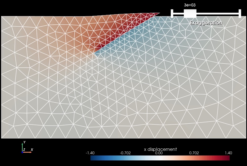
Fig. 100 Solution for Step 5a. The colors of the shaded surface indicate the x displacement, and the deformation is exaggerated by a factor of 3000. The undeformed configuration is shown by the gray wireframe.#
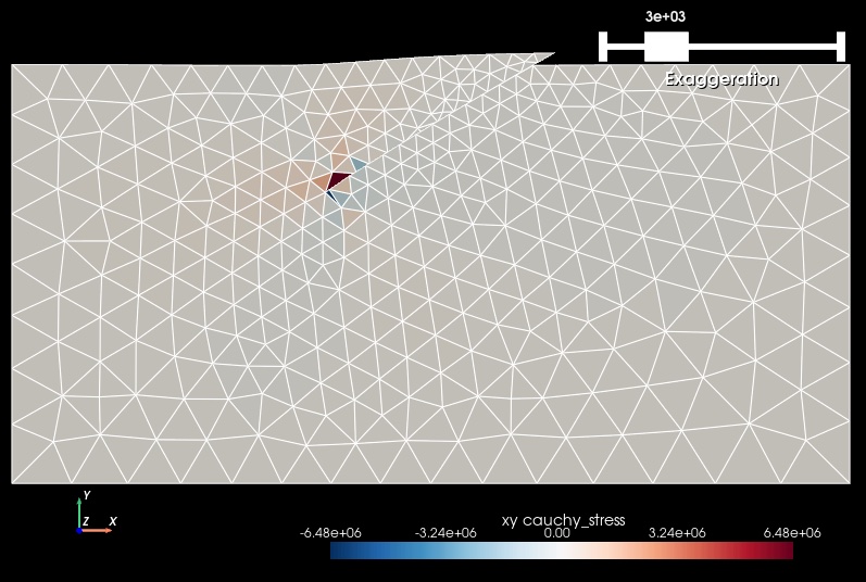
Fig. 101 Cauchy stress tensor component xy for Step 5a. The colors of the shaded surface indicate the xy component of the Cauchy stress tensor, and the deformation is exaggerated by a factor of 3000. The undeformed configuration is shown by the gray wireframe. With uniform slip on the fault, we generate a stress concentration at the buried end of the fault that is confined to just one or two cells. Thus, the stress concentration is not well resolved.#
Step 5b: Coarse Mesh#
As in some of the previous steps in this example, we refine the mesh to improve the accuracy of the results.
The parameters specific to this example are in step05b_onefault.cfg.
Simulation parameters#
We adjust the solution field to include both displacement and the Lagrange multiplier associated with the fault.
For uniform prescribed slip we use a UniformDB.
[pylithapp.mesh_generator]
refiner = pylith.topology.RefineUniform
Running the simulation#
$ pylith step05b_onefault.cfg

# The output should look very similar to Step 5a.
Visualizing the results#
In Fig. 102 and Fig. 103 we use the pylith_viz utility to visualize the simulation results.
pylith_viz --filename=output/step05b_onefault-domain.h5 warp_grid --component=x --exaggeration=3000
pylith_viz --filenames=output/step05b_onefault-crust.h5,output/step05b_onefault-wedge.h5,output/step05b_onefault-slab.h5 warp_grid --field=cauchy_stress --component=xy --exaggeration=3000

Fig. 102 Solution for Step 5b. The colors of the shaded surface indicate the x displacement, and the deformation is exaggerated by a factor of 3000. The undeformed configuration is shown by the gray wireframe.#

Fig. 103 Cauchy stress tensor component xy for Step 5b. The colors of the shaded surface indicate the xy component of the Cauchy stress tensor, and the deformation is exaggerated by a factor of 3000. The undeformed configuration is shown by the gray wireframe. Refining the mesh shows the stress concentration at the buried end of the fault is smaller in spatial extent than we observed in Step 5a. We need a higher resolution mesh to resolve the stress concentration.#
Step 5c: Coarse Mesh#
We now use higher order discretization to try to better resolve the stress concentration.
The parameters specific to this example are in step05c_onefault.cfg.
Simulation parameters#
We adjust the solution field to include both displacement and the Lagrange multiplier associated with the fault.
For uniform prescribed slip we use a UniformDB.
[pylithapp.problem]
defaults.quadrature_order = 2

[pylithapp.problem.solution.subfields]
displacement.basis_order = 2
lagrange_multiplier_fault.basis_order = 2

[pylithapp.problem.materials.slab]
derived_subfields.cauchy_strain.basis_order = 1
derived_subfields.cauchy_stress.basis_order = 1

[pylithapp.problem.materials.crust]
derived_subfields.cauchy_strain.basis_order = 1
derived_subfields.cauchy_stress.basis_order = 1

[pylithapp.problem.materials.wedge]
derived_subfields.cauchy_strain.basis_order = 1
derived_subfields.cauchy_stress.basis_order = 1
Running the simulation#
$ pylith step05c_onefault.cfg

# The output should look very similar to Steps 5a and 5b.
Visualizing the results#
In Fig. 104 and Fig. 105 we use the pylith_viz utility to visualize the simulation results.
pylith_viz --filename=output/step05c_onefault-domain.h5 warp_grid --component=x --exaggeration=3000
pylith_viz --filenames=output/step05c_onefault-crust.h5,output/step05c_onefault-wedge.h5,output/step05c_onefault-slab.h5 warp_grid --field=cauchy_stress --component=xy --exaggeration=3000

Fig. 104 Solution for Step 5c. The colors of the shaded surface indicate the x displacement, and the deformation is exaggerated by a factor of 3000. The undeformed configuration is shown by the gray wireframe.#
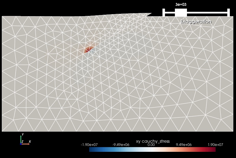
Fig. 105 Cauchy stress tensor component xy for Step 5c. The colors of the shaded surface indicate the xy component of the Cauchy stress tensor, and the deformation is exaggerated by a factor of 3000. The undeformed configuration is shown by the gray wireframe. With the higher order discretization of the solution subfields, we find better resolution of the stress concentration, which is now spread across a few cells.#
Key Points#
The displacement field is very similar for the three different discretizations.
Uniform slip generates a stress concentration at the buried end of the fault.
This stress concentration is difficult to resolve with a basis order of 1 for the solution subfields, even if we refine the mesh.
Using a basis order of 2 provides better resolution of the stress concentration, but it is poorly resolved without also refining the mesh.
Adaptive mesh refinement (not yet available in PyLith) that refines the region just around the stress concentration would help resolve the stress concentration without substantially increasing the problem size.