
Step 7: Slip on Two Faults and Maxwell Viscoelastic Materials#
Features
Triangular cells
pylith.meshio.MeshIOPetsc
pylith.problems.TimeDependent
pylith.bc.DirichletTimeDependent
spatialdata.spatialdb.SimpleDB
spatialdata.spatialdb.ZeroDB
pylith.meshio.OutputSolnBoundary
pylith.meshio.DataWriterHDF5
Quasi-static simulation
pylith.materials.Elasticity
pylith.materials.IsotropicLinearMaxwell
pylith.faults.FaultCohesiveKin
pylith.faults.KinSrcStep
spatialdata.spatialdb.UniformDB
Simulation parameters#
In this example we replace the linear, isotropic elastic bulk rheology in the slab with a linear, isotropic Maxwell viscoelastic rheology.
We use the same boundary conditions as in Step 6 but reduce the time step to resolve the viscoelastic relaxation.
The parameters specific to this example are in step07_twofaults_maxwell.cfg.
We use a very short relaxation time of 20 years, so we run the simulation for 100 years with a time step of 4 years. We use a starting time of -4 years so that the first time step will advance the solution time to 0 years.
[pylithapp.problem]
initial_dt = 4.0*year
start_time = -4.0*year
end_time = 100.0*year

normalizer.relaxation_time = 20.0*year
[pylithapp.problem.materials]
slab.bulk_rheology = pylith.materials.IsotropicLinearMaxwell

[pylithapp.problem.materials.slab]
db_auxiliary_field = spatialdata.spatialdb.SimpleDB
db_auxiliary_field.description = Maxwell viscoelastic properties
db_auxiliary_field.iohandler.filename = mat_maxwell.spatialdb

bulk_rheology.auxiliary_subfields.maxwell_time.basis_order = 0
Running the simulation#
$ pylith step07_twofaults_maxwell.cfg

# The output should look something like the following.
 >> /software/unix/py3.12-venv/pylith-debug/lib/python3.12/site-packages/pylith/apps/PyLithApp.py:77:main
 -- pylithapp(info)
 -- Running on 1 process(es).
 >> /software/unix/py3.12-venv/pylith-debug/lib/python3.12/site-packages/pylith/meshio/MeshIOObj.py:38:read
 -- meshiopetsc(info)
 -- Reading finite-element mesh
 >> /src/cig/pylith/libsrc/pylith/meshio/MeshIO.cc:85:void pylith::meshio::MeshIO::read(pylith::topology::Mesh *, const bool)
 -- meshiopetsc(info)
 -- Component 'reader': Domain bounding box:
    (-100000, 100000)
    (-100000, 0)

# -- many lines omitted --

25 TS dt 0.2 time 4.8
    0 SNES Function norm 1.848072416515e-05
    Linear solve converged due to CONVERGED_ATOL iterations 14
    1 SNES Function norm 2.259491806598e-12
  Nonlinear solve converged due to CONVERGED_FNORM_ABS iterations 1
26 TS dt 0.2 time 5.
 >> /software/unix/py3.12-venv/pylith-debug/lib/python3.12/site-packages/pylith/problems/Problem.py:199:finalize
 -- timedependent(info)
 -- Finalizing problem.
From the end of the output written to the terminal window, we see that the simulation advanced the solution 26 time steps. The PETSc TS display time in the nondimensional units, so a time of 5 corresponds to 100 years.
Visualizing the results#
In Fig. 108 we use the pylith_viz utility to visualize the x displacement field.
You can move the slider or use the p and n keys to change the increment or decrement time.
pylith_viz --filename=output/step07_twofaults_maxwell-domain.h5 warp_grid --component=x
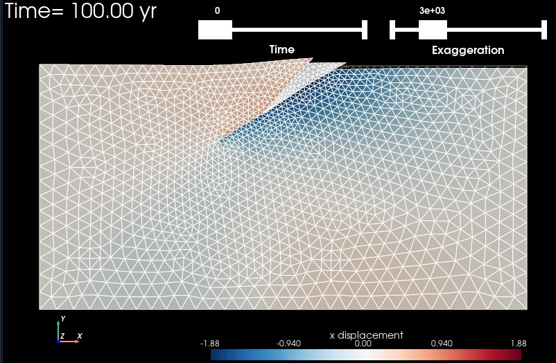
Fig. 108 Solution for Step 7 at t=100 years.
The colors of the shaded surface indicate the x displacement, and the deformation is exaggerated by a factor of 1000.
The undeformed configuration is shown by the gray wireframe.
Viscoelastic relaxation results in significant deformation in the slab material.#