
Step 2: Gravitational Body Forces with Reference Stress#
Features
Triangular cells
pylith.meshio.MeshIOPetsc
pylith.problems.TimeDependent
pylith.bc.DirichletTimeDependent
spatialdata.spatialdb.SimpleDB
spatialdata.spatialdb.ZeroDB
pylith.meshio.OutputSolnBoundary
pylith.meshio.DataWriterHDF5
Static simulation
pylith.materials.Elasticity
pylith.materials.IsotropicLinearElasticity
spatialdata.spatialdb.GravityField
Simulation parameters#
This example involves using a reference stress state to minimize the deformation when we apply the gravitational body forces.
The solution will be the perturbation from the reference state with zero displacements.
This is one method for obtaining an initial stress state associated with gravitational body forces.
We use the same roller boundary conditions that we used in Step 1.
The parameters specific to this example are in step02_gravity_refstate.cfg.
We use a reference stress state that matches the overburden (lithostatic) pressure. We have uniform material properties, so the overburden is
where compressive stress is negative.
[pylithapp.problem.materials.slab]
db_auxiliary_field.iohandler.filename = mat_gravity_refstate.spatialdb
db_auxiliary_field.query_type = linear

[pylithapp.problem.materials.slab.bulk_rheology]
use_reference_state = True

auxiliary_subfields.reference_stress.basis_order = 1
auxiliary_subfields.reference_strain.basis_order = 0
Running the simulation#
$ pylith step02_gravity_refstate.cfg

# The output should look something like the following.
 >> /software/unix/py39-venv/pylith-debug/lib/python3.9/site-packages/pylith/meshio/MeshIOObj.py:44:read
 -- meshiopetsc(info)
 -- Reading finite-element mesh
 >> /src/cig/pylith/libsrc/pylith/meshio/MeshIO.cc:94:void pylith::meshio::MeshIO::read(pylith::topology::Mesh*)
 -- meshiopetsc(info)
 -- Component 'reader': Domain bounding box:
    (-100000, 100000)
    (-100000, 0)

# -- many lines omitted --

 >> /software/unix/py39-venv/pylith-debug/lib/python3.9/site-packages/pylith/problems/TimeDependent.py:139:run
 -- timedependent(info)
 -- Solving problem.
0 TS dt 0.01 time 0.
    0 SNES Function norm 4.578015693966e-15
  Nonlinear solve converged due to CONVERGED_FNORM_ABS iterations 0
1 TS dt 0.01 time 0.01
 >> /software/unix/py39-venv/pylith-debug/lib/python3.9/site-packages/pylith/problems/Problem.py:201:finalize
 -- timedependent(info)
 -- Finalizing problem.
WARNING! There are options you set that were not used!
WARNING! could be spelling mistake, etc!
There is one unused database option. It is:
Option left: name:-ksp_converged_reason (no value)
By design we set the reference stress state so that it matches the loading from gravitational body forces in our domain with uniform material properties. As a result, the first nonlinear solver residual evaluation meets the convergence criteria. The linear solver is not used; this is why PETSc reports an unused option at the end of the simulation.
Visualizing the results#
In Fig. 88 and Fig. 89 we use the pylith_viz utility to visualize the simulation results.
pylith_viz --filenames=output/step02_gravity_refstate-domain.h5 warp_grid --exaggeration=5
pylith_viz --filenames=output/step02_gravity_refstate-crust.h5,output/step02_gravity_refstate-slab.h5,output/step02_gravity_refstate-wedge.h5 warp_grid --field=cauchy_stress --component=xy --exaggeration=5
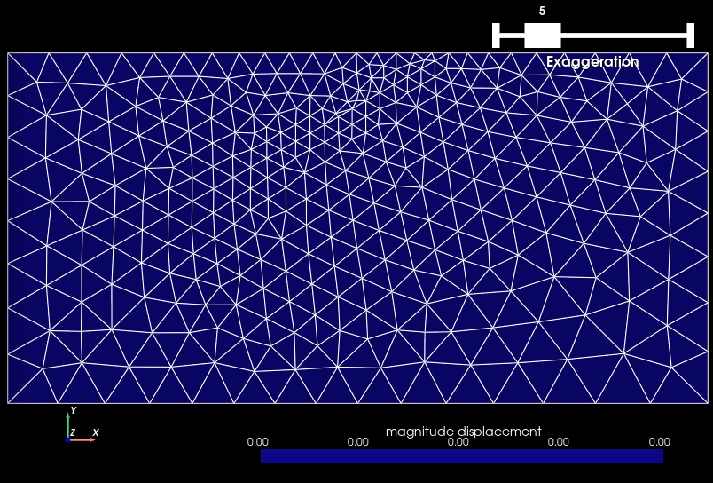
Fig. 88 Solution for Step 2. The colors of the shaded surface indicate the magnitude of the displacement, which is zero. The undeformed configuration is shown by the gray wireframe.#
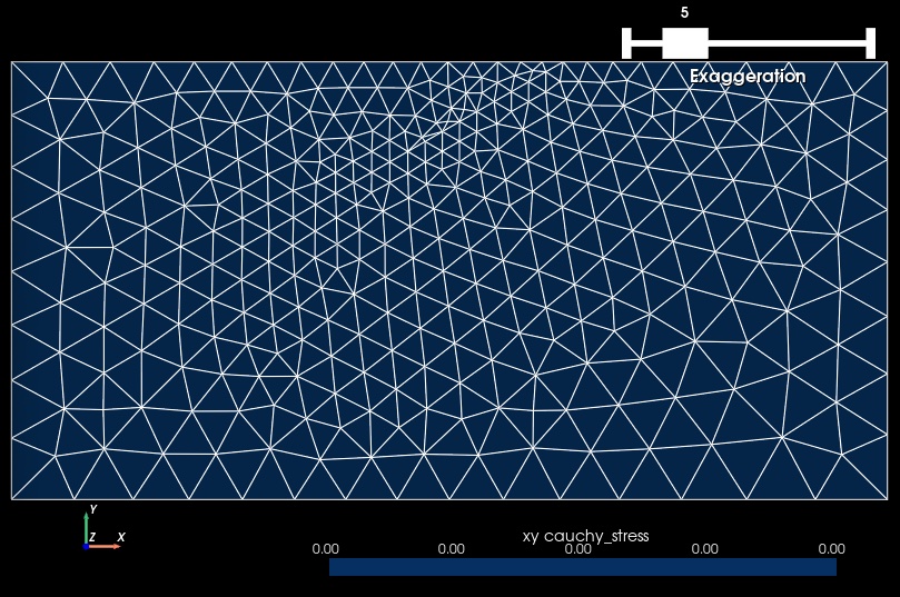
Fig. 89 Cauchy stress tensor component xy for Step 2. The colors of the shaded surface indicate the xy component of the Cauchy stress tensor, and the deformation is exaggerated by a factor of 5. The undeformed configuration is shown by the gray wireframe. The shear stress is zero.#