
Step 1: Gravitational Body Forces#
Features
Triangular cells
pylith.meshio.MeshIOPetsc
pylith.problems.TimeDependent
pylith.bc.DirichletTimeDependent
spatialdata.spatialdb.SimpleDB
spatialdata.spatialdb.ZeroDB
pylith.meshio.OutputSolnBoundary
pylith.meshio.DataWriterHDF5
Static simulation
pylith.materials.Elasticity
pylith.materials.IsotropicLinearElasticity
spatialdata.spatialdb.GravityField
This example involves a static simulation that solves for the deformation from loading by gravitational body forces. Fig. 81 shows the boundary conditions on the domain.

Fig. 81 We apply roller boundary conditions on the lateral sides and bottom of the domain.#
We solve the static elasticity equation with gravitational body forces,
Step 1a: Coarse Mesh#
Note
New in v4.1.0.
We start with a coarse resolution mesh that captures the geometry and increase the resolution of the simulation by using uniform refinement or increasing the basis order of the solution fields.
Simulation parameters#
The parameters specific to this example are in step01a_gravity.cfg.
In 2D with gravitational body forces acting in the -y direction, we need to set the direction.
[pylithapp.problem]
gravity_field = spatialdata.spatialdb.GravityField
gravity_field.gravity_dir = [0.0, -1.0, 0.0]
Running the simulation#
$ pylith step01a_gravity.cfg

# The output should look something like the following.
 >> /software/unix/py3.12-venv/pylith-debug/lib/python3.12/site-packages/pylith/meshio/MeshIOObj.py:44:read
 -- meshiopetsc(info)
 -- Reading finite-element mesh
 >> /src/cig/pylith/libsrc/pylith/meshio/MeshIO.cc:94:void pylith::meshio::MeshIO::read(topology::Mesh *)
 -- meshiopetsc(info)
 -- Component 'reader': Domain bounding box:
    (-100000, 100000)
    (-100000, 0)
 >> /software/unix/py3.12-venv/pylith-debug/lib/python3.12/site-packages/pylith/problems/Problem.py:116:preinitialize
 -- timedependent(info)
 -- Performing minimal initialization before verifying configuration.
 >> /software/unix/py3.12-venv/pylith-debug/lib/python3.12/site-packages/pylith/problems/Solution.py:44:preinitialize
 -- solution(info)
 -- Performing minimal initialization of solution.
 >> /software/unix/py3.12-venv/pylith-debug/lib/python3.12/site-packages/pylith/materials/RheologyElasticity.py:41:preinitialize
 -- isotropiclinearelasticity(info)
 -- Performing minimal initialization of elasticity rheology 'bulk_rheology'.
 >> /software/unix/py3.12-venv/pylith-debug/lib/python3.12/site-packages/pylith/materials/RheologyElasticity.py:41:preinitialize
 -- isotropiclinearelasticity(info)
 -- Performing minimal initialization of elasticity rheology 'bulk_rheology'.
 >> /software/unix/py3.12-venv/pylith-debug/lib/python3.12/site-packages/pylith/materials/RheologyElasticity.py:41:preinitialize
 -- isotropiclinearelasticity(info)
 -- Performing minimal initialization of elasticity rheology 'bulk_rheology'.
 >> /software/unix/py3.12-venv/pylith-debug/lib/python3.12/site-packages/pylith/bc/DirichletTimeDependent.py:92:preinitialize
 -- dirichlettimedependent(info)
 -- Performing minimal initialization of time-dependent Dirichlet boundary condition 'bc_xneg'.
 >> /software/unix/py3.12-venv/pylith-debug/lib/python3.12/site-packages/pylith/bc/DirichletTimeDependent.py:92:preinitialize
 -- dirichlettimedependent(info)
 -- Performing minimal initialization of time-dependent Dirichlet boundary condition 'bc_xpos'.
 >> /software/unix/py3.12-venv/pylith-debug/lib/python3.12/site-packages/pylith/bc/DirichletTimeDependent.py:92:preinitialize
 -- dirichlettimedependent(info)
 -- Performing minimal initialization of time-dependent Dirichlet boundary condition 'bc_yneg'.
 >> /software/unix/py3.12-venv/pylith-debug/lib/python3.12/site-packages/pylith/problems/Problem.py:175:verifyConfiguration
 -- timedependent(info)
 -- Verifying compatibility of problem configuration.
 >> /software/unix/py3.12-venv/pylith-debug/lib/python3.12/site-packages/pylith/problems/Problem.py:221:_printInfo
 -- timedependent(info)
 -- Scales for nondimensionalization:
    Length scale: 1000*m
    Time scale: 3.15576e+09*s
    Pressure scale: 3e+10*m**-1*kg*s**-2
    Density scale: 2.98765e+23*m**-3*kg
    Temperature scale: 1*K
 >> /software/unix/py3.12-venv/pylith-debug/lib/python3.12/site-packages/pylith/problems/Problem.py:186:initialize
 -- timedependent(info)
 -- Initializing timedependent problem with quasistatic formulation.
 >> /src/cig/pylith/libsrc/pylith/utils/PetscOptions.cc:235:static void pylith::utils::_PetscOptions::write(pythia::journal::info_t &, const char *, const pylith::utils::PetscOptions &)
 -- petscoptions(info)
 -- Setting PETSc options:
ksp_atol = 1.0e-12
ksp_converged_reason = true
ksp_error_if_not_converged = true
ksp_rtol = 1.0e-12
pc_type = lu
snes_atol = 1.0e-9
snes_converged_reason = true
snes_error_if_not_converged = true
snes_monitor = true
snes_rtol = 1.0e-12
ts_error_if_step_fails = true
ts_monitor = true
ts_type = beuler

 >> /software/unix/py3.12-venv/pylith-debug/lib/python3.12/site-packages/pylith/problems/TimeDependent.py:139:run
 -- timedependent(info)
 -- Solving problem.
0 TS dt 0.01 time 0.
    0 SNES Function norm 2.873918352757e-01
    Linear solve converged due to CONVERGED_RTOL iterations 1
    1 SNES Function norm 3.025686251687e-13
  Nonlinear solve converged due to CONVERGED_FNORM_ABS iterations 1
1 TS dt 0.01 time 0.01
 >> /software/unix/py3.12-venv/pylith-debug/lib/python3.12/site-packages/pylith/problems/Problem.py:201a:finalize
 -- timedependent(info)
 -- Finalizing problem.
At the beginning of the output written to the terminal, we see that PyLith is reading the mesh using the MeshIOPetsc reader and that it found the domain to extend from -100,000 m to +100,000 m in the x direction and from -100,000 m to 0 in the y direction.
The output also shows the scales for nondimensionalization and the PETSc options selected by PyLith.
This simulation did not use a fault, so PyLith used the LU preconditioner.
At the end of the output written to the terminal, we see that the solver advanced the solution one time step (static simulation).
The linear solve converged after 1 iterations and the norm of the residual met the relative convergence tolerance (ksp_rtol) .
The nonlinear solve converged in 1 iteration, which we expect because this is a linear problem, and the residual met the absolute convergence tolerance (snes_atol).
Visualizing the results#
The output directory contains the simulation output.
Each “observer” writes its own set of files, so the solution over the domain is in one set of files, the boundary condition information is in another set of files, and the material information is in yet another set of files.
The HDF5 (.h5) files contain the mesh geometry and topology information along with the solution fields.
The Xdmf (.xmf) files contain metadata that allow visualization tools like ParaView to know where to find the information in the HDF5 files.
To visualize the data using ParaView or Visit, load the Xdmf files.
In Fig. 82 and Fig. 83we use the pylith_viz utility to visualize the simulation results.
Because we apply the gravitational body forces to an undeformed, stress-free domain, the vertical deformation is about 2 kilometers.
pylith_viz --filenames=output/step01a_gravity-domain.h5 warp_grid --exaggeration=5
pylith_viz --filenames=output/step01a_gravity-crust.h5,output/step01a_gravity-slab.h5,output/step01a_gravity-wedge.h5 warp_grid --field=cauchy_stress --component=xy --exaggeration=5

Fig. 82 Solution for Step 1a. The colors of the shaded surface indicate the magnitude of the displacement, and the deformation is exaggerated by a factor of 5. The undeformed configuration is shown by the gray wireframe.#

Fig. 83 Cauchy stress tensor component xy for Step 1a. The colors of the shaded surface indicate the xy component of the Cauchy stress tensor, and the deformation is exaggerated by a factor of 5. The undeformed configuration is shown by the gray wireframe. We expect the shear stress (xy component) to be zero. The checkerboard pattern shows that it is close to zero on average, but there are substantial variations.#
Step 1b: Refined Mesh#
To reduce the numerical errors in the shear stress, we refine the mesh to decrease the discretization size by a factor of 2.
The parameters specific to this example are in step01b_gravity.cfg.
Simulation parameters#
We refine the mesh by setting the refiner component of the mesh_generator to pylith.topology.RefineUniform.
The default refinement is one level of refinement, which decreases the discretization size by a factor of two.
Selecting two levels of refinement would decrease the discretization size by a factor of four.
[pylithapp.mesh_generator]
refiner = pylith.topology.RefineUniform
Running the simulation#
$ pylith step01b_gravity.cfg

# The output should look very similar to that in Step 1a.
Visualizing the results#
In Fig. 84 we use the pylith_viz utility to visualize the simulation results.
pylith_viz --filenames=output/step01b_gravity-domain.h5 warp_grid --exaggeration=5
pylith_viz --filenames=output/step01b_gravity-crust.h5,output/step01b_gravity-slab.h5,output/step01b_gravity-wedge.h5 warp_grid --field=cauchy_stress --component=xy --exaggeration=5

Fig. 84 Solution for Step 1b. The colors of the shaded surface indicate the magnitude of the displacement, and the deformation is exaggerated by a factor of 5. The undeformed configuration is shown by the gray wireframe.#

Fig. 85 Cauchy stress tensor component xy for Step 1b. The colors of the shaded surface indicate the xy component of the Cauchy stress tensor, and the deformation is exaggerated by a factor of 5. The undeformed configuration is shown by the gray wireframe. Refining the mesh reduced the maximum shear stress by about a factor of 2.#
Step 1c: Higher Order Discretization#
Rather than refining the mesh further, we use a basis order of 2 for the displacement subfield in the solution.
Applying gravitational body forces without a reference stress state will result in stresses and strains that increase linearly with depth.
Consequently, the displacement field will increase with depth squared, which we can model very accurately with a basis order 2.
The parameters specific to this example are in step01c_gravity.cfg.
Simulation parameters#
Most visualization programs do not support a solution specified with coefficients for second order basis functions. The workaround is to project the solution to a basis order of 1 when we write the solution field. PyLith does this automatically. For fields that are uniform, we use a basis order of 0 to minimize memory use.
[pylithapp.problem]
defaults.quadrature_order = 2

[pylithapp.problem.solution.subfields.displacement]
basis_order = 2

[pylithapp.problem.materials.slab]
derived_subfields.cauchy_strain.basis_order = 1
derived_subfields.cauchy_stress.basis_order = 1

[pylithapp.problem.materials.crust]
derived_subfields.cauchy_strain.basis_order = 1
derived_subfields.cauchy_stress.basis_order = 1

[pylithapp.problem.materials.wedge]
derived_subfields.cauchy_strain.basis_order = 1
derived_subfields.cauchy_stress.basis_order = 1
Running the simulation#
$ pylith step01c_gravity.cfg

# The output should look very similar to that in Steps 1a and 1b.
Visualizing the results#
In Fig. 86 we use the pylith_viz utility to visualize the simulation results.
pylith_viz --filenames=output/step01c_gravity-domain.h5 warp_grid --exaggeration=5
pylith_viz --filenames=output/step01c_gravity-crust.h5,output/step01c_gravity-slab.h5,output/step01c_gravity-wedge.h5 warp_grid --field=cauchy_stress --component=xy --exaggeration=5
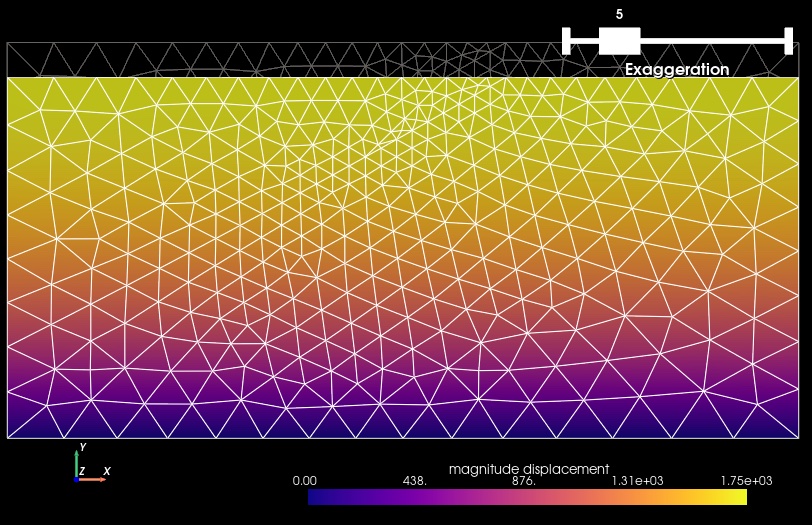
Fig. 86 Solution for Step 1c. The colors of the shaded surface indicate the magnitude of the displacement, and the deformation is exaggerated by a factor of 5. The undeformed configuration is shown by the gray wireframe.#

Fig. 87 Cauchy stress tensor component xy for Step 1c. The colors of the shaded surface indicate the xy component of the Cauchy stress tensor, and the deformation is exaggerated by a factor of 5. The undeformed configuration is shown by the gray wireframe. Increasing the basis order reduces the maximum shear stress by about 10 orders of magnitude!#
Key Points#
The displacement field is very similar for the three different discretizations.
In this case, we know the vertical displacement in the exact solution depends on the square of the depth, so we expect the numerical accuracy to be limited when we use a basis order of 1 for the displacement solution subfield.
In the exact solution, the axial components of the Cauchy stress tensor increase linearly with depth, and the xy component of the Cauchy stress is zero.
With the coarse mesh, the shear stress is close to 10 MPa throughout the mesh.
Refining the mesh decreases the magnitude shear stress by about a factor of 2.
Using a basis order of 2 for the solution subfields reduces the magnitude of the shear stress by nearly 10 orders of magnitude.
When resolving the stress field components is important, you will likely want to use a basis order of 2 for the displacement solution subfield.