
Step 4: Surface Tractions#
Features
Triangular cells
pylith.meshio.MeshIOPetsc
pylith.problems.TimeDependent
pylith.bc.DirichletTimeDependent
spatialdata.spatialdb.SimpleDB
spatialdata.spatialdb.ZeroDB
pylith.meshio.OutputSolnBoundary
pylith.meshio.DataWriterHDF5
Static simulation
pylith.materials.Elasticity
pylith.materials.IsotropicLinearElasticity
pylith.bc.NeumannTimeDependent
This example focuses on loading via surface tractions on the +y boundary. We apply tractions normal to the boundary with a trapezoidal distribution as shown in Fig. 92. We use the same roller boundary conditions that we used in Steps 1-3.

Fig. 92 We add a Neumann (traction) boundary condition on the +y boundary with roller boundary conditions on the lateral sides and bottom of the domain.#
Step 4a: Coarse Mesh#
Note
New in v4.1.0.
We start with a coarse resolution mesh that captures the geometry and increase the resolution of the simulation by using uniform refinement or increasing the basis order of the solution fields.
Simulation parameters#
The parameters specific to this example are in step04a_surfload.cfg.
[pylithapp.problem]
bc = [bc_xneg, bc_xpos, bc_yneg, bc_ypos]
bc.bc_ypos = pylith.bc.NeumannTimeDependent

[pylithapp.problem.bc.bc_ypos]
label = boundary_ypos
label_value = 13

db_auxiliary_field = spatialdata.spatialdb.SimpleDB
db_auxiliary_field.description = Neumann BC +y edge
db_auxiliary_field.iohandler.filename = traction_surfload.spatialdb

db_auxiliary_field.query_type = linear

auxiliary_subfields.initial_amplitude.basis_order = 1
Running the simulation#
$ pylith step04a_surfload.cfg

# The output should look something like the following.
 >> /software/unix/py3.12-venv/pylith-debug/lib/python3.12/site-packages/pylith/apps/PyLithApp.py:77:main
 -- pylithapp(info)
 -- Running on 1 process(es).
 >> /software/unix/py3.12-venv/pylith-debug/lib/python3.12/site-packages/pylith/meshio/MeshIOObj.py:38:read
 -- meshiopetsc(info)
 -- Reading finite-element mesh
 >> /src/cig/pylith/libsrc/pylith/meshio/MeshIO.cc:85:void pylith::meshio::MeshIO::read(pylith::topology::Mesh *, const bool)
 -- meshiopetsc(info)
 -- Component 'reader': Domain bounding box:
    (-100000, 100000)
    (-100000, 0)

# -- many lines omitted --

 >> /software/unix/py3.12-venv/pylith-debug/lib/python3.12/site-packages/pylith/problems/TimeDependent.py:132:run
 -- timedependent(info)
 -- Solving problem.
0 TS dt 0.01 time 0.
    0 SNES Function norm 1.213351093160e-02
    Linear solve converged due to CONVERGED_ATOL iterations 1
    1 SNES Function norm 1.008881341134e-15
  Nonlinear solve converged due to CONVERGED_FNORM_ABS iterations 1
1 TS dt 0.01 time 0.01
 >> /software/unix/py3.12-venv/pylith-debug/lib/python3.12/site-packages/pylith/problems/Problem.py:199:finalize
 -- timedependent(info)
 -- Finalizing problem.
As expected from the use of the LU preconditioner and linear problem, both the linear and nonlinear solvers converged in 1 iteration.
Visualizing the results#
In Fig. 93 and Fig. 94 we use the pylith_viz utility to visualize the simulation results.
pylith_viz --filenames=output/step04a_surfload-domain.h5 warp_grid --exaggeration=500
pylith_viz --filenames=output/step04a_surfload-crust.h5,output/step04a_surfload-slab.h5,output/step04a_surfload-wedge.h5 warp_grid --field=cauchy_stress --component=xy --exaggeration=500
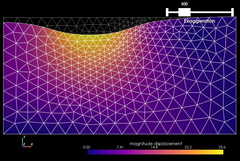
Fig. 93 Solution for Step 4a. The colors of the shaded surface indicate the magnitude of the displacement, and the deformation is exaggerated by a factor of 500. The undeformed configuration is shown by the gray wireframe.#
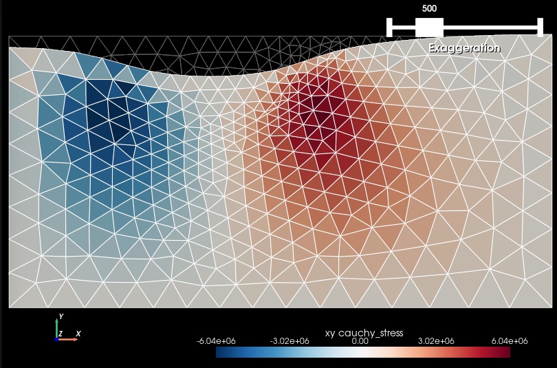
Fig. 94 Cauchy stress tensor component xy for Step 4a. The colors of the shaded surface indicate the xy component of the Cauchy stress tensor, and the deformation is exaggerated by a factor of 500. The undeformed configuration is shown by the gray wireframe. We observe that the coarse resolution mesh does not resolve the shear stress very well, and we have moderate jumps in the shear stress field between adjacent cells.#
Step 4b: Refined Mesh#
As in Step 1, we try to improve on the accuracy of the solution by refining the mesh.
Simulation parameters#
The parameters specific to this example are in step04b_surfload.cfg.
[pylithapp.mesh_generator]
refiner = pylith.topology.RefineUniform
Running the simulation#
$ pylith step04b_surfload.cfg

# The output should look very similar to Step 4a.
Visualizing the results#
In Fig. 95 and Fig. 96 we use the pylith_viz utility to visualize the simulation results.
pylith_viz --filename=output/step04b_surfload-domain.h5 warp_grid --exaggeration=500
pylith_viz --filenames=output/step04b_surfload-crust.h5,output/step04b_surfload-slab.h5,output/step04b_surfload-wedge.h5 warp_grid --field=cauchy_stress --component=xy --exaggeration=500

Fig. 95 Solution for Step 4b. The colors of the shaded surface indicate the magnitude of the displacement, and the deformation is exaggerated by a factor of 500. The undeformed configuration is shown by the gray wireframe.#

Fig. 96 Cauchy stress tensor component xy for Step 4b. The colors of the shaded surface indicate the xy component of the Cauchy stress tensor, and the deformation is exaggerated by a factor of 500. The undeformed configuration is shown by the gray wireframe. Refining the mesh reduces the size of the jumps in the shear stress field between adjacent cells.#
Step 4c: Higher Order Discretization#
As in Step 1, we again use a higher order discretization of the solution field to improve the accuracy of the model.
Simulation parameters#
The parameters specific to this example are in step04c_surfload.cfg.
[pylithapp.problem]
defaults.quadrature_order = 2

[pylithapp.problem.solution.subfields.displacement]
basis_order = 2

[pylithapp.problem.materials.slab]
derived_subfields.cauchy_strain.basis_order = 1
derived_subfields.cauchy_stress.basis_order = 1

[pylithapp.problem.materials.crust]
derived_subfields.cauchy_strain.basis_order = 1
derived_subfields.cauchy_stress.basis_order = 1

[pylithapp.problem.materials.wedge]
derived_subfields.cauchy_strain.basis_order = 1
derived_subfields.cauchy_stress.basis_order = 1
Running the simulation#
$ pylith step04c_surfload.cfg

# The output should look very similar to Steps 4a and 4b.
Visualizing the results#
In Fig. 97 and Fig. 98 we use the pylith_viz utility to visualize the simulation results.
pylith_viz --filename=output/step04c_surfload-domain.h5 warp_grid --exaggeration=500
pylith_viz --filenames=output/step04c_surfload-crust.h5,output/step04c_surfload-slab.h5,output/step04c_surfload-wedge.h5 warp_grid --field=cauchy_stress --component=xy --exaggeration=500

Fig. 97 Solution for Step 4c. The colors of the shaded surface indicate the magnitude of the displacement, and the deformation is exaggerated by a factor of 500. The undeformed configuration is shown by the gray wireframe.#

Fig. 98 Cauchy stress tensor component xy for Step 4c. The colors of the shaded surface indicate the xy component of the Cauchy stress tensor, and the deformation is exaggerated by a factor of 500. The undeformed configuration is shown by the gray wireframe. The higher order discretization removes the jumps in the shear stress field between adjacent cells.#
Key Points#
The displacement field is very similar for the three different discretizations.
This stress field, especially the shear stress component, is not well resolved with a basis order of 1 and the coarse mesh.
Refining the mesh to decrease the discretization size by a factor of two yields better resolution of the shear stress field.
Using a basis order of 2 with the coarse mesh provides better resolution of the stress concentration compared with refining the mesh.
When resolving the stress field components is important, you will likely want to use a basis ordre of 2 for the displacement solution subfield.