
Step 3: Gravitational Body Forces with Incompressible Elasticity#
Features
Triangular cells
pylith.meshio.MeshIOPetsc
pylith.problems.TimeDependent
pylith.bc.DirichletTimeDependent
spatialdata.spatialdb.SimpleDB
spatialdata.spatialdb.ZeroDB
pylith.meshio.OutputSolnBoundary
pylith.meshio.DataWriterHDF5
Static simulation
pylith.materials.IncompressibleElasticity
spatialdata.spatialdb.GravityField
field split preconditioner
Schur complement preconditioner
Simulation parameters#
In this example we use incompressible elasticity (see Incompressible Isotropic Elasticity with Infinitesimal Strain (Bathe) for the finite-element formulation) to obtain the stress field associated with gravitational body forces,
Because the material is incompressible and the material is confined on the lateral boundaries and bottom, we do not expect any deformation.
In general, this is a more robust way to determine an initial stress state for gravitational body forces compared to using a reference stress state, especially when the material properties are not uniform.
We use the same roller boundary conditions that we used in Steps 1 and 2.
The parameters specific to this example are in step03_gravity_incompressible.cfg.
solution = pylith.problems.SolnDispPres

[pylithapp.problem.materials]
slab = pylith.materials.IncompressibleElasticity
crust = pylith.materials.IncompressibleElasticity
wedge = pylith.materials.IncompressibleElasticity

[pylithapp.problem.materials.slab]
db_auxiliary_field.iohandler.filename = mat_elastic_incompressible.spatialdb

[pylithapp.problem.materials.crust]
db_auxiliary_field.iohandler.filename = mat_elastic_incompressible.spatialdb

[pylithapp.problem.materials.wedge]
db_auxiliary_field.iohandler.filename = mat_elastic_incompressible.spatialdb
With pressure as a solution subfield, we add a Dirichlet boundary condition to set the confining pressure to 0 on the ground surface (+y boundary).
[pylithapp.problem]
bc = [bc_xneg, bc_xpos, bc_yneg, bc_ypos]
bc.bc_ypos = pylith.bc.DirichletTimeDependent

[pylithapp.problem.bc.bc_ypos]
label = boundary_ypos
label_value = 13
constrained_dof = [0]
field = pressure
db_auxiliary_field = pylith.bc.ZeroDB
db_auxiliary_field.description = Dirichlet BC for pressure on +y edge

auxiliary_subfields.initial_amplitude.basis_order = 0

observers.observer.data_fields = [pressure]
Running the simulation#
$ pylith step03_gravity_incompressible.cfg

# The output should look something like the following.
 >> /software/unix/py38-venv/pylith-debug/lib/python3.8/site-packages/pylith/meshio/MeshIOObj.py:44:read
 -- meshiopetsc(info)
 -- Reading finite-element mesh
 >> /src/cig/pylith/libsrc/pylith/meshio/MeshIO.cc:94:void pylith::meshio::MeshIO::read(pylith::topology::Mesh*)
 -- meshiopetsc(info)
 -- Component 'reader': Domain bounding box:
    (-100000, 100000)
    (-100000, 0)

# -- many lines omitted --

 >> /src/cig/pylith/libsrc/pylith/utils/PetscOptions.cc:235:static void pylith::utils::_PetscOptions::write(pythia::journal::info_t &, const char *, const pylith::utils::PetscOptions &)
 -- petscoptions(info)
 -- Setting PETSc options:
ksp_atol = 1.0e-12
ksp_converged_reason = true
ksp_error_if_not_converged = true
ksp_rtol = 1.0e-12
pc_fieldsplit_schur_factorization_type = full
snes_atol = 1.0e-9
snes_converged_reason = true
snes_error_if_not_converged = true
snes_monitor = true
snes_rtol = 1.0e-12
ts_error_if_step_fails = true
ts_monitor = true
ts_type = beuler

 >> /src/cig/pylith/libsrc/pylith/utils/PetscOptions.cc:235:static void pylith::utils::_PetscOptions::write(pythia::journal::info_t &, const char *, const pylith::utils::PetscOptions &)
 -- petscoptions(info)
 -- Ignoring PETSc options (already set):
fieldsplit_displacement_pc_type = lu
fieldsplit_pressure_pc_type = lu
pc_fieldsplit_schur_precondition = full
pc_fieldsplit_type = schur
pc_type = fieldsplit

 >> /software/unix/py39-venv/pylith-debug/lib/python3.9/site-packages/pylith/meshio/MeshIOObj.py:44:read
 -- timedependent(info)
 -- Solving problem.
0 TS dt 0.01 time 0.
    0 SNES Function norm 4.866941773461e-01
    Linear solve converged due to CONVERGED_ATOL iterations 1
    1 SNES Function norm 3.099989574301e-13
  Nonlinear solve converged due to CONVERGED_FNORM_ABS iterations 1
1 TS dt 0.01 time 0.01
 >> /software/unix/py39-venv/pylith-debug/lib/python3.9/site-packages/pylith/problems/Problem.py:201:finalize
 -- timedependent(info)
 -- Finalizing problem.
PyLith detected use of incompressible elasticity, so it selected a field split preconditioner with an LU preconditioner for each of the solution subfields as described in PETSc Options. As a result, the linear solve converged in 1 iterations.
Visualizing the results#
In Fig. 90 and Fig. 91 we use the pylith_viz utility to visualize the simulation results.
pylith_viz --filename=output/step03_gravity_incompressible-domain.h5 warp_grid --exaggeration=5
pylith_viz --filenames=output/step03_gravity_incompressible-crust.h5,output/step03_gravity_incompressible-slab.h5,output/step03_gravity_incompressible-wedge.h5 warp_grid --field=cauchy_stress --component=xy --exaggeration=5
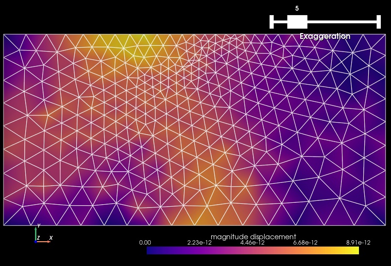
Fig. 90 Solution for Step 3. The colors of the shaded surface indicate the magnitude of the displacement. The undeformed configuration is shown by the gray wireframe. There is negligible deformation and the stress state (not shown) matches the one in Step 2.#
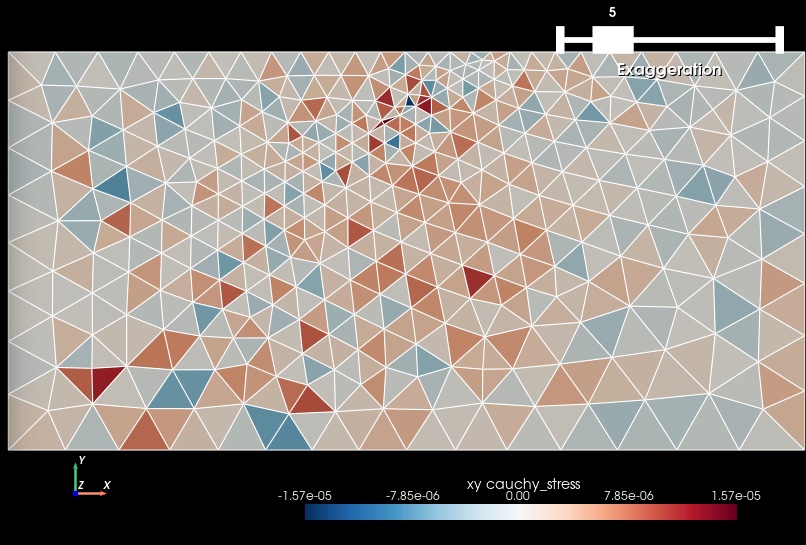
Fig. 91 Cauchy stress tensor component xy for Step 3. The colors of the shaded surface indicate the xy component of the Cauchy stress tensor, and the deformation is exaggerated by a factor of 5. The undeformed configuration is shown by the gray wireframe. The shear stress is negligible.#