Step 2: Single Earthquake Rupture and Velocity Boundary Conditions

Features

• Triangular cells

• pylith.meshio.MeshIOPetsc

• pylith.problems.TimeDependent

• pylith.materials.Elasticity

• pylith.materials.IsotropicLinearElasticity

• pylith.faults.FaultCohesiveKin

• pylith.faults.KinSrcStep

• field split preconditioner

• Schur complement preconditioner

• pylith.bc.DirichletTimeDependent

• spatialdata.spatialdb.UniformDB

• pylith.meshio.OutputSolnBoundary

• pylith.meshio.DataWriterHDF5

• Quasi-static simulation

• spatialdata.spatialdb.SimpleDB

Simulation parameters

This example involves a quasi-static simulation that solves for the deformation from velocity boundary conditions and prescribed coseismic slip on the fault. We let strain accumulate due to the motion of the boundaries and then release the strain by prescribing 2 meters of right-lateral slip at t=100 years. Fig. 56 shows the boundary conditions on the domain. The parameters specific to this example are in step02_slip_velbc.cfg.

Fig. 56 Boundary conditions for quasistatic simulation with velocity boundary conditions and coseismic slip. We set the x displacement to zero on the +x and -x boundaries. We set the y velocity to -1 cm/yr on the +x boundary and +1 cm/yr on the -x boundary. We prescribe 2 meters of right-lateral slip to occur at 100 years to release the accumulated strain energy.

Listing 77 Time stepping parameters for Step 2.

[pylithapp.problem]
initial_dt = 5.0*year
start_time = -5.0*year
end_time = 120.0*year

Boundary conditions

We switch the Dirichlet boundary conditions from specifying an initial amplitude to specifying a constant velocity,

(173)\[\begin{align} \dot{u}_x(-50km,y) &= 0,\\ \dot{u}_y(-50km,y) &= +1 cm/yr,\\ \dot{u}_x(+50km,y) &= 0,\\ \dot{u}_y(+50km,y) &= -1 cm/yr. \end{align}\]

Listing 78 Dirichlet boundary conditions for Step 2. We only show the details for the +x boundary.

[pylithapp.problem.bc.bc_xpos]
use_initial = False
use_rate = True

db_auxiliary_field = spatialdata.spatialdb.SimpleDB
db_auxiliary_field.description = Dirichlet BC +x boundary
db_auxiliary_field.iohandler.filename = disprate_bc_xpos.spatialdb

As in Step 1 we prescribe 2.0 meters of right-lateral slip, but in this case we set slip to occur at t=100 years.

Listing 79 Prescribed slip parameters for Step 2.

[pylithapp.problem.interfaces.fault.eq_ruptures.rupture]
db_auxiliary_field = spatialdata.spatialdb.UniformDB
db_auxiliary_field.description = Fault rupture auxiliary field spatial database
db_auxiliary_field.values = [initiation_time, final_slip_left_lateral, final_slip_opening]
db_auxiliary_field.data = [100.0*year, -2.0*m, 0.0*m]

Running the simulation

Listing 80 Run Step 2 simulation

$ pylith step02_slip_velbc.cfg

# The output should look something like the following.
 >> /software/unix/py39-venv/pylith-debug/lib/python3.9/site-packages/pylith/meshio/MeshIOObj.py:44:read
 -- meshiopetsc(info)
 -- Reading finite-element mesh
 >> /src/cig/pylith/libsrc/pylith/meshio/MeshIO.cc:94:void pylith::meshio::MeshIO::read(topology::Mesh *)
 -- meshiopetsc(info)
 -- Component 'reader': Domain bounding box:
    (-50000, 50000)
    (-75000, 75000)

# -- many lines omitted --

24 TS dt 0.05 time 1.15
    0 SNES Function norm 5.390420823432e-04
    Linear solve converged due to CONVERGED_ATOL iterations 29
    1 SNES Function norm 1.250412952119e-12
  Nonlinear solve converged due to CONVERGED_FNORM_ABS iterations 1
25 TS dt 0.05 time 1.2
 >> /software/unix/py39-venv/pylith-debug/lib/python3.9/site-packages/pylith/problems/Problem.py:201:finalize
 -- timedependent(info)
 -- Finalizing problem.

The beginning of the output written to the terminal is identical to that from Step 1. At the end of the output, we see that the simulation advanced the solution 25 time steps. Remember that the PETSc TS monitor shows the nondimensionalized time and time step values.

Visualizing the results

In Fig. 57 we use ParaView to visualize the x displacement field using the viz/plot_dispwarp.py Python script. First, we start ParaView from the examples/strikeslip-2d directory.

Listing 81 Open ParaView using the command line.

$ PATH_TO_PARAVIEW/paraview

# For macOS, it will be something like
$ /Applications/ParaView-5.10.1.app/Contents/MacOS/paraview

Next, we override the default name of the simulation file with the name of the current simulation.

Listing 82 Set the simulation in the ParaView Python Shell.

>>> SIM = "step02_slip_velbc"

Finally, we run the viz/plot_dispwarp.py Python script as described in ParaView Python Scripts.

Tip

You can use the “play” button to animate the solution in time.

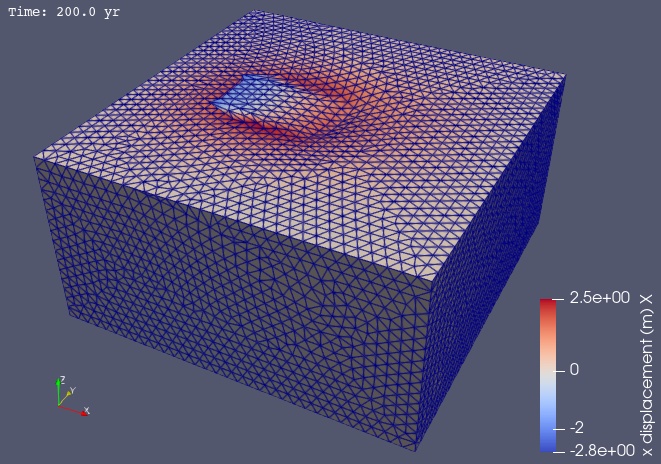
Fig. 57 Solution for Step 2 at t=100 yr. The colors of the shaded surface indicate the magnitude of the y displacement, and the deformation is exaggerated by a factor of 1000. The undeformed configuration is show by the gray wireframe. The coseismic fault slip at 100 years releases all of the accumulated strain energy.