Subduction Zone (3D)

The files are in the directory examples/subduction-3d. The files and directories for this set of examples includes:

README.md:

README file containing a brief description of the various examples.

*.cfg:

PyLith parameter files.

cubit_*.jou:

Files used to construct the finite-element mesh using Cubit.

*.spatialdb:

Spatial database filesFiles associated with the spatial databases.

utils:

Directory containing Python scripts for pre- and post-processing.

viz:

Directory containing ParaView Python scripts and other files for visualizing results.

input:

Directory for simulation input data that must be downloaded.

output:

Directory containing simulation output. It is created automatically when running the simulations.

scratch:

Directory for temporary files generated by utility scripts.

Overview

This suite of examples demonstrates use of a wide variety of features and the general workflow often used in research simulations. We base the model on the Cascadia subduction zone (Fig. 99). These examples focus on modeling the deformation associated with the the subducting slab, including interseismic deformation with aseismic slip (creep) and viscoelastic relaxation, coseismic slip on the slab interface and a splay fault, and slow slip events on the subduction interface. We account for the 3D material properties associated with different elastic properties for the subducting slab, mantle, continental crust, and accretionary wedge. To keep the computation time in these examples short, we limit our model to an 800 km \(\times\) 800 km \(\times\) 400 km domain and we use a relatively coarse discretization. For simplicity and to reduce complexity in constructing the mesh, we use a flat top surface (elevation of 0 with respect to mean sea level).

Fig. 99 Cartoon of the Cascadia Subduction Zone showing the subduction of the Juan de Fuca Plate under the North American Plate. Source - U.S. Geological Survey Fact Sheet 060-00

Fig. 100 shows our conceptual model with a slab, mantle, continental crust, and accretionary wedge. We cut off the slab at a depth of 100 km. We use a transverse geographic projection coordinate system with Portland, Oregon, as the origin to georeference our model. To model the motion of the slab, we include a fault for the subduction interface (the interface between the top of the slab and the mantle, crust, and wedge), as well as a fault between the bottom of the slab and the mantle.

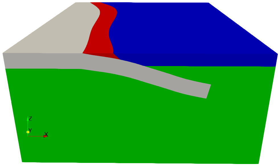
Fig. 100 Conceptual model based on the Cascadia Subduction Zone. The model includes the subduction slab (white), the mantle (green), continental crust (blue), and an accretionary wedge (red).

Step 1:

Static axial compression.

Step 2:

Quasi-static coseismic and postseismic deformation from an earthquake rupture in the center of the subduction zone interface.

Step 3:

Quasi-static interseisic deformation with creep on the top and bottom of the slab.

Step 4:

Quasi-static earthquake cycle with prescribed earthquake rupture and creep.

Warning

Steps 5-8 are still being updated for use with PyLith v3.

Danger

These simulations are significantly larger than those for the other suites of examples. Some of the time-dependent simulations may take 30 minutes or more to run and use up to 4 GB of memory. We are working to select better preconditioners to improve the solvers and reduce the runtime.

Example Workflow

• Cubit Mesh
  • Setup
  • Meshing using Journal Scripts
  • Visualizing the Mesh
• Common Information
• Step 1: Axial Compression
  • Simulation parameters
  • Visualizing the results
• Step 2: Earthquake Rupture and Postseismic Relaxation
  • Simulation parameters
  • Visualizing the results
• Step 3: Interseismic Deformation
  • Simulation parameters
  • Visualizing the results
• Step 4: Earthquake Cycle with Prescribed Slip
  • Simulation parameters
  • Visualizing the results
• Suggested Exercises