Step 8: Slip on Two Faults and Power-law Viscoelastic Materials#

Features

Triangular cells
pylith.meshio.MeshIOPetsc
pylith.problems.TimeDependent
pylith.bc.DirichletTimeDependent
spatialdata.spatialdb.SimpleDB
spatialdata.spatialdb.ZeroDB
pylith.meshio.OutputSolnBoundary
pylith.meshio.DataWriterHDF5
Quasi-static simulation
pylith.materials.Elasticity
pylith.materials.IsotropicPowerLaw
pylith.faults.FaultCohesiveKin
pylith.faults.KinSrcStep
spatialdata.spatialdb.UniformDB
spatialdata.spatialdb.CompositeDB

Simulation parameters#

In this example we replace the linear, isotropic Maxwell viscoelastic bulk rheology in the slab in Step 7 with an isotropic powerlaw viscoelastic rheology. The other parameters remain the same as those in Step 6. The parameters specific to this example are in step08_twofaults_powerlaw.cfg.

Listing 134 Power-law viscoelastic bulk rheology parameters for Step 8.#

[pylithapp.problem.materials]
slab.bulk_rheology = pylith.materials.IsotropicPowerLaw

[pylithapp.problem.materials.slab]
db_auxiliary_field = spatialdata.spatialdb.CompositeDB
db_auxiliary_field.description = Power law material properties

bulk_rheology.auxiliary_subfields.power_law_reference_strain_rate.basis_order = 0
bulk_rheology.auxiliary_subfields.power_law_reference_stress.basis_order = 0
bulk_rheology.auxiliary_subfields.power_law_exponent.basis_order = 0

[pylithapp.problem.materials.slab.db_auxiliary_field]
# Elastic properties
values_A = [density, vs, vp]
db_A = spatialdata.spatialdb.SimpleDB
db_A.description = Elastic properties for slab
db_A.iohandler.filename = mat_elastic.spatialdb

# Power law properties
values_B = [
	 power_law_reference_stress,  power_law_reference_strain_rate,  power_law_exponent,
	 viscous_strain_xx, viscous_strain_yy, viscous_strain_zz, viscous_strain_xy,
	 reference_stress_xx, reference_stress_yy, reference_stress_zz, reference_stress_xy,
	 reference_strain_xx, reference_strain_yy, reference_strain_zz, reference_strain_xy,
	 deviatoric_stress_xx,  deviatoric_stress_yy,  deviatoric_stress_zz,  deviatoric_stress_xy
	 ]
db_B = spatialdata.spatialdb.SimpleDB
db_B.description = Material properties specific to power law bulk rheology for the slab
db_B.iohandler.filename = mat_powerlaw.spatialdb
db_B.query_type = linear

Power-law spatial database#

New in v4.0.0

We use the utility script pylith_powerlaw_gendb (see pylith_powerlaw_gendb) to generate the spatial database mat_powerlaw.spatialdb with the power-law bulk rheology parameters. We provide the parameters for pylith_powerlaw_gendb in powerlaw_gendb.cfg, which follows the same formatting conventions as the PyLith parameter files.

Listing 135 Generate spatial database with power-law viscoelastic material properties.#

$ pylith_powerlaw_gendb powerlaw_gendb.cfg

Running the simulation#

Listing 136 Run Step 8 simulation#

$ pylith step08_twofaults_powerlaw.cfg

# The output should look something like the following.
 >> /software/unix/py39-venv/pylith-debug/lib/python3.9/site-packages/pylith/meshio/MeshIOObj.py:44:read
 -- meshiopetsc(info)
 -- Reading finite-element mesh
 >> /src/cig/pylith/libsrc/pylith/meshio/MeshIO.cc:94:void pylith::meshio::MeshIO::read(pylith::topology::Mesh*)
 -- meshiopetsc(info)
 -- Component 'reader': Domain bounding box:
    (-100000, 100000)
    (-100000, 0)

# -- many lines omitted --

25 TS dt 0.2 time 4.8
    0 SNES Function norm 2.142894498538e-06
    Linear solve converged due to CONVERGED_ATOL iterations 200
    1 SNES Function norm 6.320401896875e-09
    Linear solve converged due to CONVERGED_ATOL iterations 67
    2 SNES Function norm 1.048498421861e-10
  Nonlinear solve converged due to CONVERGED_FNORM_ABS iterations 2
26 TS dt 0.2 time 5.
 >> /software/baagaard/py38-venv/pylith-debug/lib/python3.8/site-packages/pylith/problems/Problem.py:201:finalize
 -- timedependent(info)
 -- Finalizing problem.

As in Step 7, the simulation advances 26 time steps. With a nonlinear bulk rheology, the nonlinear solver now requires several iterations to converge at each time step.

Visualizing the results#

The output directory contains the simulation output. Each “observer” writes its own set of files, so the solution over the domain is in one set of files, the boundary condition information is in another set of files, and the material information is in yet another set of files. The HDF5 (.h5) files contain the mesh geometry and topology information along with the solution fields. The Xdmf (.xmf) files contain metadata that allow visualization tools like ParaView to know where to find the information in the HDF5 files. To visualize the data using ParaView or Visit, load the Xdmf files.

In Fig. 86 we use ParaView to visualize the y displacement field using the viz/plot_dispwarp.py Python script. First, we start ParaView from the examples/reverse-2d directory. Before running the viz/plot_dispwarp.py Python script as described in ParaView Python Scripts, we set the simulation name in the ParaView Python Shell.

Listing 137 Set the simulation and exaggeration in the ParaView Python Shell.#

>>> SIM = "step08_twofaults_powerlaw"
>>> FIELD_COMPONENT = "X"

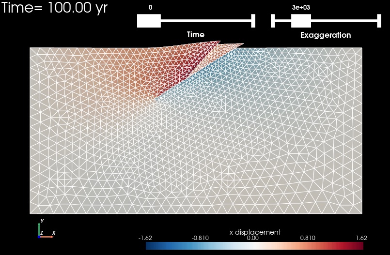
Solution for Step 8. The colors indicate the magnitude of the x displacement, and the deformation is exaggerated by a factor of 1000. — Fig. 86 Solution for Step 8 at t=100 years. The colors of the shaded surface indicate the magnitude of the x displacement, and the deformation is exaggerated by a factor of 1000. The undeformed configuration is show by the gray wireframe. Our parameters for the power-law bulk rheology result in much less viscoelastic relaxation in this case compared to Step 7.#