
Step 6: Slip on Two Faults and Elastic Materials#
Features
Triangular cells
pylith.meshio.MeshIOPetsc
pylith.problems.TimeDependent
pylith.bc.DirichletTimeDependent
spatialdata.spatialdb.SimpleDB
spatialdata.spatialdb.ZeroDB
pylith.meshio.OutputSolnBoundary
pylith.meshio.DataWriterHDF5
Static simulation
pylith.materials.Elasticity
pylith.materials.IsotropicLinearElasticity
pylith.faults.FaultCohesiveKin
pylith.faults.KinSrcStep
spatialdata.spatialdb.UniformDB
In this example we add coseismic slip on the splay fault with an origin time of 40 years.
We specify 2 meters of reverse slip on the main fault and 1 meter of reverse slip on the splay fault.
Fig. 107 shows the boundary conditions on the domain.
The parameters specific to this example are in step06_twofaults-elastic.cfg.

Fig. 107 Boundary conditions for static coseismic slip on both the main and splay faults. We prescribe 2 meters of reverse slip on the main fault with 1 meter of reverse slip on the splay fault. We use roller boundary conditions on the lateral sides and bottom of the domain.#
Simulation parameters#
We use uniform refinement to reduce the discretization size by a factor of 2 and increase the numerical resolution. With different origin times for slip on the two faults, we need to add time stepping. With a linearly elastic, quasistatic model (no inertia) and fixed displacements on the boundaries, the displacement field only changes as a result of fault slip, so we can use just a few time steps to resolve the deformation. We impose slip on the main fault in the first time step (advancing the solution to t=0), and impose slip on the splay fault in the third time step (advancing the solution to t=40 years).
[pylithapp.mesh_generator]
refiner = pylith.topology.RefineUniform

[pylithapp.problem]
initial_dt = 20.0*year
start_time = -20.0*year
end_time = 40.0*year
Important
In 2D simulations slip is specified in terms of opening and left-lateral components. This provides a consistent, unique sense of slip that is independent of the fault orientation. For our geometry in this example, right lateral slip corresponds to reverse slip on both of the dipping faults.
Important
Both faults contain one end that is buried within the domain. The splay fault ends where it meets the main fault. When PyLith inserts cohesive cells into a mesh with buried edges (in this case a point), we must identify these buried edges so that PyLith properly adjusts the topology along these edges.
For properly topology of the cohesive cells, the main fault must be listed first in the array of faults so that it will be created before the splay fault.
We create an array of 2 faults, which are FaultCohesiveKin by default, and use UniformDB objects to specify uniform reverse slip on each fault.
[pylithapp.problem]
interfaces = [fault, splay]

[pylithapp.problem.interfaces.fault]
label = fault
label_value = 20

observers.observer.data_fields = [slip, traction_change]

[pylithapp.problem.interfaces.fault.eq_ruptures.rupture]
db_auxiliary_field = spatialdata.spatialdb.UniformDB
db_auxiliary_field.description = Fault rupture for main fault
db_auxiliary_field.values = [initiation_time, final_slip_left_lateral, final_slip_opening]
db_auxiliary_field.data = [0.0*s, -2.0*m, 0.0*m]

[pylithapp.problem.interfaces.splay]
label = splay
label_value = 22

observers.observer.data_fields = [slip, traction_change]

[pylithapp.problem.interfaces.splay.eq_ruptures.rupture]
db_auxiliary_field = spatialdata.spatialdb.UniformDB
db_auxiliary_field.description = Fault rupture for splay fault
db_auxiliary_field.values = [initiation_time, final_slip_left_lateral, final_slip_opening]
db_auxiliary_field.data = [0.0*s, -1.0*m, 0.0*m]
Running the simulation#
$ pylith step06_twofaults_elastic.cfg

# The output should look something like the following.
>> software/pylith-debug/lib/python3.12/site-packages/pylith/apps/PyLithApp.py:79:main
-- info (application-flow)
-- Running on 1 process(es).

# -- many lines omitted --
>> src/cig/pylith/libsrc/pylith/problems/TimeDependent.cc:473:void pylith::problems::TimeDependent::solve()
-- info (application-flow)
-- Component 'timedependent.problem': Solving equations.
0 TS dt 0.2 time -0.2
    0 SNES Function norm 9.084511105523e+00
      Linear solve converged due to CONVERGED_ATOL iterations 14
    1 SNES Function norm 5.480772341407e-08
    Nonlinear solve converged due to CONVERGED_FNORM_ABS iterations 1
1 TS dt 0.2 time 0.
    0 SNES Function norm 5.480772341407e-08
    Nonlinear solve converged due to CONVERGED_FNORM_ABS iterations 0
2 TS dt 0.2 time 0.2
    0 SNES Function norm 3.245094761897e+00
      Linear solve converged due to CONVERGED_ATOL iterations 13
    1 SNES Function norm 3.950115997088e-08
    Nonlinear solve converged due to CONVERGED_FNORM_ABS iterations 1
3 TS dt 0.2 time 0.4
>> software/pylith-debug/lib/python3.12/site-packages/pylith/problems/Problem.py:222:finalize
-- info (application-flow)
-- Finalizing problem.
From the end of the output written to the terminal window, we see that the linear solver converged in 13-14 iterations and met the absolute convergence tolerance (ksp_atol).
As we expect for this linear problem, the nonlinear solver converged in 1 iteration.
Visualizing the results#
In Fig. 108 we use the pylith_viz utility to visualize the x displacement field.
pylith_viz --filenames=output/step06_twofaults_elastic-domain.h5 warp_grid --component=x --exaggeration=3000
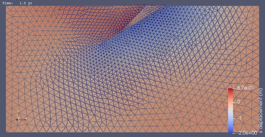
Fig. 108 Solution for Step 6 at t=40 yr. The colors of the shaded surface indicate the x displacement, and the deformation is exaggerated by a factor of 1000. The undeformed configuration is shown by the gray wireframe.#