
Step 2: Magma inflation with evolution of porosity#
New in v4.0.0.
Features
Quasi-static problem
LU preconditioner
pylith.materials.Poroelasticity
pylith.meshio.MeshIOPetsc
pylith.problems.TimeDependent
pylith.problems.SolnDispPresTracStrain
pylith.problems.InitialConditionDomain
pylith.bc.DirichletTimeDependent
pylith.bc.NeumannTimeDependent
pylith.meshio.DataWriterHDF5
spatialdata.spatialdb.SimpleGridDB
spatialdata.spatialdb.UniformDB
Poroelasticity with porosity state variable
Isotropic linear poroelasticity with reference state
Simulation parameters#
We extend the simulation in Step 1 by including evolution of the porosity, which depends on the time derivative of the pressure and trace strain. We also compute the deformation relative to a uniform reference compressive pressure of 5 MPa to illustrate how to use a reference state with poroelasticity. We use the same initial conditions and boundary conditions as in Step 1.
Because the evolution of porosity depends on the time derivative of the solution subfields, we need to include the time derivatives in the solution field. As a result, we have 6 subfields in our solution field.
# Poroelasticity with porosity state variable requires solution with time derivatives
solution = pylith.problems.SolnDispPresTracStrainVelPdotTdot

# Set basis order for all solution subfields
[pylithapp.problem.solution.subfields]
displacement.basis_order = 2
pressure.basis_order = 1
trace_strain.basis_order = 1
velocity.basis_order = 2
pressure_t.basis_order = 1
trace_strain_t.basis_order = 1
[pylithapp.problem.materials.crust]
use_state_variables = True

db_auxiliary_field.values = [
    solid_density, fluid_density, fluid_viscosity, porosity, shear_modulus, drained_bulk_modulus, biot_coefficient, fluid_bulk_modulus, solid_bulk_modulus, isotropic_permeability,
    reference_stress_xx, reference_stress_yy, reference_stress_zz, reference_stress_xy,
    reference_strain_xx, reference_strain_yy, reference_strain_zz, reference_strain_xy
    ]
db_auxiliary_field.data   = [
    2500*kg/m**3, 1000*kg/m**3, 0.001*Pa*s, 0.01, 6.0*GPa, 10.0*GPa, 1.0, 2.0*GPa, 20.0*GPa, 1e-15*m**2,
    -5.0*MPa, -5.0*MPa, -5.0*MPa, 0.0*MPa,
    0.0, 0.0, 0.0, 0.0
    ]

auxiliary_subfields.porosity.basis_order = 1

[pylithapp.problem.materials.crust.bulk_rheology]
use_reference_state = True


[pylithapp.problem.materials.intrusion]
use_state_variables = True

db_auxiliary_field.values = [
    solid_density, fluid_density, fluid_viscosity, porosity, shear_modulus, drained_bulk_modulus, biot_coefficient, fluid_bulk_modulus, solid_bulk_modulus, isotropic_permeability,
    reference_stress_xx, reference_stress_yy, reference_stress_zz, reference_stress_xy,
    reference_strain_xx, reference_strain_yy, reference_strain_zz, reference_strain_xy
    ]
db_auxiliary_field.data   = [
    2500*kg/m**3,  1000*kg/m**3, 0.001*Pa*s, 0.1, 6.0*GPa, 10.0*GPa, 0.8, 2.0*GPa, 20.0*GPa, 1e-13*m**2,
    -5.0*MPa, -5.0*MPa, -5.0*MPa, 0.0*Pa,
    0.0, 0.0, 0.0, 0.0
    ]

auxiliary_subfields.porosity.basis_order = 1

[pylithapp.problem.materials.intrusion.bulk_rheology]
use_reference_state = True
The changes in the physics as well as the default solver settings that impact the initial guess leads to a large initial residual at the second time step. Consequently, we increase the divergence tolerance for the linear solver.
[pylithapp.petsc]
# Increase divergence tolerance. Initial guess at second time step is not accurate.
ksp_divtol = 1.0e+5
Running the simulation#
$ pylith step02_inflation_statevars.cfg

# The output should look something like the following.
>> software/pylith-debug/lib/python3.12/site-packages/pylith/apps/PyLithApp.py:76:main
-- info (application-flow)
-- Running on 1 process(es).
>> software/pylith-debug/lib/python3.12/site-packages/pylith/utils/PetscManager.py:64:showOptions
-- info (application-flow)
-- PETSc user options:
    ksp_divtol = 1.0e+6

# -- many lines omitted --

50 TS dt 0.151476 time 7.42235
    0 SNES Function norm 1.207876038262e-02
      Linear solve converged due to CONVERGED_ATOL iterations 79
    1 SNES Function norm 6.174330339004e-09
    Nonlinear solve converged due to CONVERGED_FNORM_ABS iterations 1
51 TS dt 0.151476 time 7.57382
>> software/pylith-debug/lib/python3.12/site-packages/pylith/problems/Problem.py:222:finalize
-- info (application-flow)
-- Finalizing problem.
The linear solver exhibits similar performance with less than 50 iterations at most time steps. Furthermore, the problem is still linear, so the nonlinear solver converges in one iteration.
Visualizing the results#
In Fig. 171 we use the pylith_viz utility to visualize the pressure field.
You can move the slider or use the p and n keys to change the increment or decrement time.
pylith_viz --filenames=output/step02_inflation_statevars-domain.h5 warp_grid --field=pressure
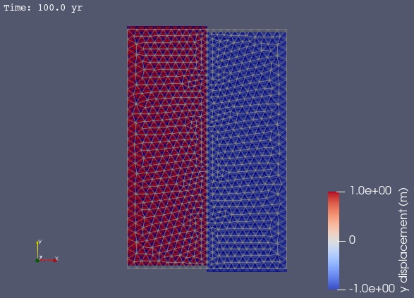
Fig. 171 Solution for Step 2 at t=100 yr. The colors of the shaded surface indicate the fluid pressure, and the deformation is exaggerated by a factor of 1000. The reference state gives rise to greater vertical deformation compared to Step 1. The choice of material properties does not lead to significant changes in porosity in either material during the simulation (not shown in the figure).#