
Step 1: Magma inflation#
Features
Quasi-static problem
LU preconditioner
pylith.materials.Poroelasticity
pylith.meshio.MeshIOPetsc
pylith.problems.TimeDependent
pylith.problems.SolnDispPresTracStrain
pylith.problems.InitialConditionDomain
pylith.bc.DirichletTimeDependent
pylith.bc.NeumannTimeDependent
pylith.meshio.DataWriterHDF5
spatialdata.spatialdb.SimpleGridDB
spatialdata.spatialdb.UniformDB
Simulation parameters#
This example uses poroelasticity to model flow of magma up through a conduit and into a magma reservoir.
The magma reservoir and conduit have a higher permeability than the surrounding crust.
We generate flow by imposing a pressure on the external boundary of the conduit that is higher than the uniform initial pressure in the domain.
Fig. 168 shows the boundary conditions on the domain.
The parameters specific to this example are in step01_inflation.cfg.

Fig. 168 Boundary and initial conditions for magma inflation. We apply roller boundary conditions on the +x, -x, and -y boundaries. We impose zero pressure (undrained conditions) on the +y boundary and a pressure on the external boundary of the conduit to generate fluid flow.#
[pylithapp.timedependent]
start_time = -0.2*year
initial_dt = 0.2*year
end_time = 10.0*year
[pylithapp.problem]
ic = [domain]
ic.domain = pylith.problems.InitialConditionDomain

[pylithapp.problem.ic.domain]
subfields = [pressure]
db = spatialdata.spatialdb.SimpleDB
db.description = Initial conditions for domain
db.iohandler.filename = initial_pressure.spatialdb
We create an array of 5 Dirichlet boundary conditions: 3 for displacement and 2 for fluid pressure. We have zero displacement perpendicular to the -x, +x, and -y boundaries, zero pressure on the +y boundary, and 10 MPa of fluid pressure on the external boundary of the conduit.
[pylithapp.problem]
bc = [bc_xneg, bc_xpos, bc_yneg, bc_ypos, bc_flow]

bc.bc_xneg = pylith.bc.DirichletTimeDependent
bc.bc_xpos = pylith.bc.DirichletTimeDependent
bc.bc_yneg = pylith.bc.DirichletTimeDependent
bc.bc_ypos = pylith.bc.DirichletTimeDependent
bc.bc_flow = pylith.bc.DirichletTimeDependent

[pylithapp.problem.bc.bc_xneg]
constrained_dof = [0]
label = boundary_xneg
field = displacement
db_auxiliary_field = pylith.bc.ZeroDB
db_auxiliary_field.description = Dirichlet BC -x

[pylithapp.problem.bc.bc_xpos]
constrained_dof = [0]
label = boundary_xpos
field = displacement
db_auxiliary_field = pylith.bc.ZeroDB
db_auxiliary_field.description = Dirichlet BC +x

[pylithapp.problem.bc.bc_yneg]
constrained_dof = [1]
label = boundary_yneg
field = displacement
db_auxiliary_field = pylith.bc.ZeroDB
db_auxiliary_field.description = Dirichlet BC -y

[pylithapp.problem.bc.bc_ypos]
constrained_dof = [0]
label = boundary_ypos
field = pressure
db_auxiliary_field = pylith.bc.ZeroDB
db_auxiliary_field.description = Dirichlet BC +z

[pylithapp.problem.bc.bc_flow]
constrained_dof = [0]
label = boundary_flow
field = pressure
db_auxiliary_field = spatialdata.spatialdb.UniformDB
db_auxiliary_field.description = Flow into external boundary of conduit
db_auxiliary_field.values = [initial_amplitude]
db_auxiliary_field.data = [10.0*MPa]
Running the simulation#
$ pylith step01_inflation.cfg

# The output should look something like the following.
>> software/pylith-debug/lib/python3.12/site-packages/pylith/apps/PyLithApp.py:80:main
-- info (application-flow)
-- Running on 1 process(es).
>> src/cig/pylith/libsrc/pylith/utils/PetscOptions.cc:251:static void pylith::utils::_PetscOptions::write(pythia::journal::info_t &, const char *, const PetscOptions &)
-- info (application-flow)
-- Setting PETSc options:
    fieldsplit_displacement_pc_type = lu
    fieldsplit_pressure_pc_type = bjacobi
    fieldsplit_trace_strain_pc_type = bjacobi
    ksp_atol = 1.0e-7
    ksp_converged_reason = true
    ksp_error_if_not_converged = true
    ksp_guess_pod_size = 8
    ksp_guess_type = pod
    ksp_rtol = 1.0e-14
    pc_fieldsplit_0_fields = 2
    pc_fieldsplit_1_fields = 1
    pc_fieldsplit_2_fields = 0
    pc_fieldsplit_type = multiplicative
    pc_type = fieldsplit
    snes_atol = 5.0e-7
    snes_converged_reason = true
    snes_error_if_not_converged = true
    snes_monitor = true
    snes_rtol = 1.0e-14
    ts_error_if_step_fails = true
    ts_exact_final_time = matchstep
    ts_monitor = true
    ts_type = beuler
    viewer_hdf5_collective = true
>> src/cig/pylith/libsrc/pylith/meshio/MeshIOPetsc.cc:205:virtual void pylith::meshio::MeshIOPetsc::_read()
-- info (application-flow)
-- Component 'meshiopetsc.reader': Reading finite-element mesh from 'mesh_tri.msh'.
>> src/cig/pylith/libsrc/pylith/meshio/MeshIO.cc:76:void pylith::meshio::MeshIO::read(pylith::topology::Mesh *, const bool)
-- info (application-flow)
-- Component 'meshiopetsc.reader': Domain bounding box:
    (0, 20000)
    (-20000, 0)
>> src/cig/pylith/libsrc/pylith/problems/TimeDependent.cc:316:virtual void pylith::problems::TimeDependent::verifyConfiguration() const
-- info (application-flow)
-- Component 'timedependent.problem': Verifying problem configuration.
>> software/pylith-debug/lib/python3.12/site-packages/pylith/problems/Problem.py:238:_printInfo
-- info (application-flow)
-- Scales for nondimensionalization:
    Length scale: 5000*m
    Displacement scale: 10*m
    Time scale: 4.16667e+07*s
    Rigidity scale: 6e+09*m**-1*kg*s**-2
    Temperature scale: 1*K
>> src/cig/pylith/libsrc/pylith/problems/TimeDependent.cc:342:virtual void pylith::problems::TimeDependent::initialize()
-- info (application-flow)
-- Component 'timedependent.problem': Initializing problem.
>> src/cig/pylith/libsrc/pylith/problems/TimeDependent.cc:473:void pylith::problems::TimeDependent::solve()
-- info (application-flow)
-- Component 'timedependent.problem': Solving equations.
0 TS dt 0.151476 time -0.151476
    0 SNES Function norm 9.951368195027e-01
      Linear solve converged due to CONVERGED_ATOL iterations 160
    1 SNES Function norm 3.315089885638e-08
    Nonlinear solve converged due to CONVERGED_FNORM_ABS iterations 1

# -- many lines omitted --

50 TS dt 0.151476 time 7.42235
    0 SNES Function norm 1.755481622154e-03
      Linear solve converged due to CONVERGED_ATOL iterations 44
    1 SNES Function norm 3.243946411840e-08
    Nonlinear solve converged due to CONVERGED_FNORM_ABS iterations 1
51 TS dt 0.151476 time 7.57382
>> software/pylith-debug/lib/python3.12/site-packages/pylith/problems/Problem.py:222:finalize
-- info (application-flow)
-- Finalizing problem.
At the beginning of the output written to the terminal, we see that PyLith is reading the mesh using the MeshIOPetsc reader and that it found the domain to extend from 0 to 20 km in the x direction and from -20 km to 0 in the y direction.
PyLith detects the use of poroelasticity without a fault and selects appropriate preconditioning options as discussed in PETSc Options.
At the end of the output written to the terminal, we see that the solver advanced the solution 51 time steps.
The linear solver converges in about 50 or less iteration at most time steps and the norm of the residual met the absolute convergence tolerance (ksp_atol) .
The nonlinear solve converged in 1 iteration, which we expect because this is a linear problem, and the residual met the absolute convergence tolerance (snes_atol).
Visualizing the results#
In Fig. 169 we use the pylith_viz utility to visualize the pressure field.
You can move the slider or use the p and n keys to change the increment or decrement time.
The initial linear variation in fluid pressure adjusts to match the boundary conditions and spatial variations in constitutive behavior.
pylith_viz --filenames=output/step01_inflation-domain.h5 warp_grid --field=pressure
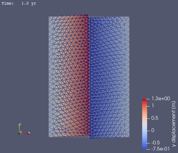
Fig. 169 Solution for Step 1 at t=100 yr. The colors of the shaded surface indicate the fluid pressure, and the deformation is exaggerated by a factor of 1000.#
Step 1b: Adaptive Time Stepping#
In Step 1b we demonstrate the use adaptive time stepping. We start with an initial time step of 0.2 years and let the adaptive time stepping algorithm increase the time step as the rate of deformation decreases. We dcrease the tolerances slightly (the default tolerances are 0.05) for better agreement with the solution from uniform time stepping.
[pylithapp.timedependent]
start_time = -0.2*year
initial_dt = 0.2*year
end_time = 10.0*year

petsc_defaults.adaptive_time_stepping = True

[pylithapp.petsc]
ts_atol = 0.02
ts_rtol = 0.02
$ pylith step01_inflation.cfg step01b_inflation.cfg

# The output should look something like the following.
>> software/pylith-debug/lib/python3.12/site-packages/pylith/utils/PetscManager.py:55:initialize
-- info (application-flow)
-- Initialized PETSc with user options
    ts_atol = 0.02
    ts_rtol = 0.02
>> software/pylith-debug/lib/python3.12/site-packages/pylith/apps/PyLithApp.py:80:main
-- info (application-flow)
-- Running on 1 process(es).
>> src/cig/pylith/libsrc/pylith/utils/PetscOptions.cc:251:static void pylith::utils::_PetscOptions::write(pythia::journal::info_t &, const char *, const PetscOptions &)
-- info (application-flow)
-- Setting PETSc options:
    fieldsplit_displacement_pc_type = lu
    fieldsplit_pressure_pc_type = bjacobi
    fieldsplit_trace_strain_pc_type = bjacobi
    ksp_atol = 1.0e-7
    ksp_converged_reason = true
    ksp_error_if_not_converged = true
    ksp_guess_pod_size = 8
    ksp_guess_type = pod
    ksp_rtol = 1.0e-14
    pc_fieldsplit_0_fields = 2
    pc_fieldsplit_1_fields = 1
    pc_fieldsplit_2_fields = 0
    pc_fieldsplit_type = multiplicative
    pc_type = fieldsplit
    snes_atol = 5.0e-7
    snes_converged_reason = true
    snes_error_if_not_converged = true
    snes_monitor = true
    snes_rtol = 1.0e-14
    ts_adapt_monitor = true
    ts_adapt_reject_safety = 0.1
    ts_adapt_safety = 0.2
    ts_adapt_type = basic
    ts_error_if_step_fails = true
    ts_exact_final_time = matchstep
    ts_monitor = true
    ts_type = beuler
    viewer_hdf5_collective = true

# -- many lines omitted --

19 TS dt 1.2231 time 6.35073
    0 SNES Function norm 1.893597646523e-03
      Linear solve converged due to CONVERGED_ATOL iterations 77
    1 SNES Function norm 2.064447881404e-08
    Nonlinear solve converged due to CONVERGED_FNORM_ABS iterations 1
  TSAdapt basic beuler 0: step  19 accepted t=6.35073    + 1.223e+00 dt=1.412e+00  wlte= 0.03  wltea=   -1 wlter=   -1
20 TS dt 1.41194 time 7.57382
>> software/pylith-debug/lib/python3.12/site-packages/pylith/problems/Problem.py:222:finalize
-- info (application-flow)
-- Finalizing problem.
The adaptive time stepping algorithm shortens a few of the early time steps but then lengthens the time step as the rate of deformation decreases. We end up with 20 time steps with adaptive time stepping compared to 51 with uniform time steps.
./plot_compare.py

Fig. 170 Vertical displacement and fluid pressure time histories for Step 1 and 1b at locations with the largest changes. We find very little difference between the solutions from uniform time stepping (51 time steps) and adaptive time stepping (20 time steps).#