
Step 2: Shear Displacement#
Features
Tetrahedral cells
pylith.meshio.MeshIOPetsc
pylith.problems.TimeDependent
pylith.materials.Elasticity
pylith.materials.IsotropicLinearElasticity
spatialdata.spatialdb.UniformDB
pylith.meshio.OutputSolnBoundary
pylith.meshio.DataWriterHDF5
Static simulation
LU preconditioner
pylith.bc.DirichletTimeDependent
spatialdata.spatialdb.SimpleDB
spatialdata.spatialdb.ZeroDB
Simulation parameters#
This example corresponds to shear deformation due to Dirichlet (displacement) boundary conditions.
We apply Dirichlet (displacement) boundary conditions for the y displacement on the +x (boundary_xpos) and -x (boundary_xneg) boundaries and for the x displacement on the +y (boundary_ypos) and -y (boundary_yneg) boundaries.
Fig. 40 shows the boundary conditions on the domain.
The parameters specific to this example are in step02_sheardisp.cfg.

Fig. 42 Boundary conditions for shear deformation. We constrain the y displacement on the +x and -x boundaries and the x displacement on the +y and -y boundaries.#
We create an array of 5 Dirichlet boundary conditions. On the -x, +x, -y, and +y boundaries we impose shear displacement.
bc = [bc_xneg, bc_xpos, bc_yneg, bc_ypos, bc_zneg]
bc.bc_xneg = pylith.bc.DirichletTimeDependent
bc.bc_xpos = pylith.bc.DirichletTimeDependent
bc.bc_yneg = pylith.bc.DirichletTimeDependent
bc.bc_ypos = pylith.bc.DirichletTimeDependent
bc.bc_zneg = pylith.bc.DirichletTimeDependent

[pylithapp.problem.bc.bc_xneg]
label = boundary_xneg
label_value = 10
constrained_dof = [1]

db_auxiliary_field = spatialdata.spatialdb.SimpleDB
db_auxiliary_field.description = Dirichlet BC -x boundary
db_auxiliary_field.iohandler.filename = sheardisp_bc_xneg.spatialdb
db_auxiliary_field.query_type = linear
Running the simulation#
$ pylith step02_sheardisp.cfg

# The output should look something like the following.
>> software/pylith-debug/lib/python3.12/site-packages/pylith/apps/PyLithApp.py:79:main
-- info (application-flow)
-- Running on 1 process(es).

# -- many lines omitted --
>> software/unix/py39-venv/pylith-debug/lib/python3.9/site-packages/pylith/problems/TimeDependent.py:139:run
-- timedependent(info)
-- Solving problem.
0 TS dt 0.001 time 0.
    0 SNES Function norm 5.433645185324e-01
      Linear solve converged due to CONVERGED_ATOL iterations 4
    1 SNES Function norm 4.280274905934e-09
    Nonlinear solve converged due to CONVERGED_FNORM_ABS iterations 1
1 TS dt 0.001 time 0.001
>> software/unix/py39-venv/pylith-debug/lib/python3.9/site-packages/pylith/problems/Problem.py:201:finalize
-- timedependent(info)
-- Finalizing problem.
WARNING! There are options you set that were not used!
WARNING! could be spelling mistake, etc!
There is one unused database option. It is:
Option left: name:-mg_levels_pc_type value: pbjacobi source: code
The output written to the terminal is nearly identical to what we saw for Step 1.
Visualizing the results#
In Fig. 43 we use the pylith_viz utility to visualize the x displacement field.
pylith_viz --filenames=output/step02_sheardisp-domain.h5 warp_grid --component=x
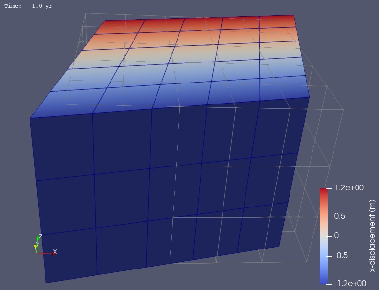
Fig. 43 Solution for Step 2. The colors of the shaded surface indicate the x displacement, and the deformation is exaggerated by a factor of 1000. The undeformed configuration is shown by the gray wireframe.#