Step 2: Shear Displacement

Features

• Quadrilateral cells

• pylith.meshio.MeshIOAscii

• pylith.problems.TimeDependent

• pylith.materials.Elasticity

• pylith.materials.IsotropicLinearElasticity

• spatialdata.spatialdb.UniformDB

• pylith.meshio.DataWriterHDF5

• Static simulation

• LU preconditioner

• pylith.bc.DirichletTimeDependent

• spatialdata.spatialdb.SimpleDB

Simulation parameters

This example corresponds to shear deformation due to Dirichlet (displacement) boundary conditions. We apply Dirichlet (displacement) boundary conditions for the y displacement on the +x (boundary_xpos) and -x (boundary_xneg) boundaries and for the x displacement on the +y (boundary_ypos) and -y (boundary_yneg) boundaries. Fig. 26 shows the boundary conditions on the domain. The parameters specific to this example are in step02_sheardisp.cfg.

Fig. 28 Boundary conditions for shear deformation. We constrain the y displacement on the +x and -x boundaries and the x displacement on the +y and -y boundaries.

We create an array of 4 DirichletTimeDependent boundary conditions. For each of these boundary conditions we must specify which degrees of freedom are constrained, the name of the label marking the boundary (name of the group of vertices in the finite-element mesh file), and the values for the Dirichlet boundary condition. The displacement field varies along each boundary, so we use a SimpleDB spatial database and the linear query type.

Listing 27 Specifying the boundary conditions for Step 2. We only show the detailed settings for the -x boundary.

[pylithapp.problem]
bc = [bc_xneg, bc_yneg, bc_xpos, bc_ypos]
bc.bc_xneg = pylith.bc.DirichletTimeDependent
bc.bc_yneg = pylith.bc.DirichletTimeDependent
bc.bc_xpos = pylith.bc.DirichletTimeDependent
bc.bc_ypos = pylith.bc.DirichletTimeDependent
        
# Degree of freedom (dof) 1 corresponds to y displacement. 
constrained_dof = [1]
label = boundary_xneg
db_auxiliary_field = spatialdata.spatialdb.SimpleDB
db_auxiliary_field.description = Dirichlet BC -x edge
db_auxiliary_field.iohandler.filename = sheardisp_bc_xneg.spatialdb
db_auxiliary_field.query_type = linear

Running the simulation

Listing 28 Run Step 2 simulation

$ pylith step02_sheardisp.cfg

# The output should look something like the following.
 >> /software/unix/py39-venv/pylith-debug/lib/python3.9/site-packages/pylith/meshio/MeshIOObj.py:44:read
 -- meshioascii(info)
 -- Reading finite-element mesh
 >> /src/cig/pylith/libsrc/pylith/meshio/MeshIO.cc:94:void pylith::meshio::MeshIO::read(topology::Mesh *)
 -- meshioascii(info)
 -- Component 'reader': Domain bounding box:
    (-6000, 6000)
    (-16000, -0)

# -- many lines omitted --

 >> /software/unix/py39-venv/pylith-debug/lib/python3.9/site-packages/pylith/problems/TimeDependent.py:139:run
 -- timedependent(info)
 -- Solving problem.
0 TS dt 0.01 time 0.
    0 SNES Function norm 2.239977678460e-03 
    Linear solve converged due to CONVERGED_ATOL iterations 1
    1 SNES Function norm 1.964321818484e-18 
  Nonlinear solve converged due to CONVERGED_FNORM_ABS iterations 1
1 TS dt 0.01 time 0.01
 >> /software/unix/py39-venv/pylith-debug/lib/python3.9/site-packages/pylith/problems/Problem.py:201:finalize
 -- timedependent(info)
 -- Finalizing problem.

The output written to the terminal is nearly identical to what we saw for Step 1. We omit the middle portion of the output which shows that the domain, the scales for nondimensionalization, and PETSc options all remain the same.

Visualizing the results

In Fig. 29 we use ParaView to visualize the x displacement field using the viz/plot_dispwarp.py Python script. First, we start ParaView from the examples/box-2d directory.

Listing 29 Open ParaView using the command line.

$ PATH_TO_PARAVIEW/paraview

# For macOS, it will be something like
$ /Applications/ParaView-5.10.1.app/Contents/MacOS/paraview

Next, we override the default name of the simulation file with the name of the current simulation.

Listing 30 Set the simulation in the ParaView Python Shell.

>>> SIM = "step02_sheardisp"

Finally, we run the viz/plot_dispwarp.py Python script as described in ParaView Python Scripts.

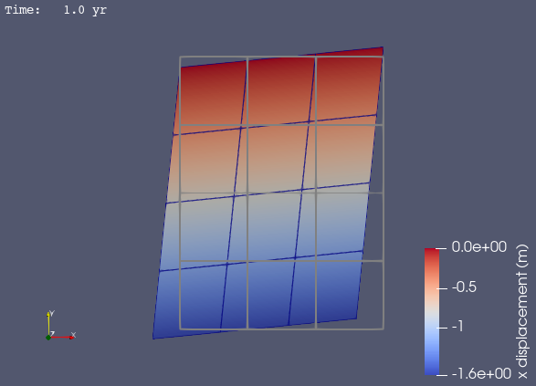
Fig. 29 Solution for Step 2. The colors of the shaded surface indicate the magnitude of the x displacement, and the deformation is exaggerated by a factor of 1000. The undeformed configuration is show by the gray wireframe.