Step 5: Green’s Functions

Features

• Triangular cells

• pylith.meshio.MeshIOPetsc

• pylith.problems.TimeDependent

• pylith.materials.Elasticity

• pylith.materials.IsotropicLinearElasticity

• pylith.faults.FaultCohesiveKin

• pylith.faults.KinSrcStep

• field split preconditioner

• Schur complement preconditioner

• pylith.bc.DirichletTimeDependent

• spatialdata.spatialdb.UniformDB

• pylith.meshio.OutputSolnBoundary

• pylith.meshio.DataWriterHDF5

• “Green’s functions”

• Fault slip impulses

Simulation parameters

In this example we compute static Green’s functions for fault slip and use then in Step 6 to invert for fault slip. We generated the “observations” for the slip inversion in Step 4.

We impose fault slip impulses over the central portion of the strike-slip fault (-25 km \(\le\) y \(\le\) +25km), which is slightly larger than where we specified coseismic in Step 4. Fig. 69 summarizes the boundary conditions and fault slip. The parameters specific to this example are in step05_greensfns.cfg.

Fig. 69 Boundary conditions for static Green’s functions. We set the x and y displacement to zero on the +x and -x boundaries and prescribe left-lateral slip impulses.

We use the GreensFns problem and specify the fault on which to impose fault slip impulses. As in Step 4, we include output at the fake GNSS stations using OutputSolnPoints. In the fault interfaces section we set the fault type to FaultCohesiveImpulses for our fault where we want to impose fault slip impulses for the Green’s functions. We also use a spatial database to limit the section of the fault where we impose the fault slip impulses to -25 km \(\le\) y \(\le\) +25 km.

Important

Currently, a basis order of 1 (default) for the slip auxiliary subfield is the only choice that gives accurate results in a slip inversion due to the factors described here.

The basis order for the slip auxiliary subfield controls the representation of the slip field for the impulses. For a given impulse, a basis order of 1 will impose unit slip at a vertex with zero slip at all other vertices. Likewise, a basis order of 0 will attempt to impose unit slip over a cell with zero slip in all other cells; however, this creates a jump in slip at the cell boundaries that cannot be accurately represented by the finite-element solution. As a result, you should not use a basis order of 0 for the slip auxiliary field. A basis order of 2 will impose slip at vertices as well as edge degrees of freedom in the cell. Because PyLith output decimates the basis order to 0 or 1, you should avoid this choice of basis order as well until we provide better ways to output fields discretized with higher order basis functions.

Listing 92 Parameters for computing static Green’s functions for fault slip impulses. We change the problem type and specify the fault on which we apply the slip impulses.

[pylithapp]
problem = pylith.problems.GreensFns

[pylithapp.greensfns]
label = fault
label_value = 20

Listing 93 Parameters for the slip impulses. We change the fault type and limit the impulses to the lateral slip component.

[pylithapp.problem.interfaces]
fault = pylith.faults.FaultCohesiveImpulses

[pylithapp.problem.interfaces.fault]
impulse_dof = [1]

db_auxiliary_field = spatialdata.spatialdb.SimpleDB
db_auxiliary_field.description = Fault rupture auxiliary field spatial database
db_auxiliary_field.iohandler.filename = slip_impulses.spatialdb

auxiliary_subfields.slip.basis_order = 1

Running the simulation

Listing 94 Run Step 5 simulation

$  pylith step05_greensfns.cfg

# The output should look something like the following.
 >> /software/unix/py3.12-venv/pylith-debug/lib/python3.12/site-packages/pylith/apps/PyLithApp.py:77:main
 -- pylithapp(info)
 -- Running on 1 process(es).
 >> /software/unix/py3.12-venv/pylith-debug/lib/python3.12/site-packages/pylith/meshio/MeshIOObj.py:38:read
 -- meshiopetsc(info)
 -- Reading finite-element mesh
 >> /src/cig/pylith/libsrc/pylith/meshio/MeshIO.cc:85:void pylith::meshio::MeshIO::read(pylith::topology::Mesh *, const bool)
 -- meshiopetsc(info)
 -- Component 'reader': Domain bounding box:
    (-50000, 50000)
    (-75000, 75000)

# -- many lines omitted --

 >> /src/cig/pylith/libsrc/pylith/problems/GreensFns.cc:322:void pylith::problems::GreensFns::solve()
 -- greensfns(info)
 -- Component 'problem': Computing Green's function 12 of 12.
  0 SNES Function norm 3.027654014246e-03
  Linear solve converged due to CONVERGED_ATOL iterations 18
  1 SNES Function norm 1.850212226728e-12
Nonlinear solve converged due to CONVERGED_ITS iterations 1
 >> /software/unix/py3.12-venv/pylith-debug/lib/python3.12/site-packages/pylith/problems/Problem.py:199:finalize
 -- greensfns(info)
 -- Finalizing problem.
WARNING! There are options you set that were not used!
WARNING! could be spelling mistake, etc!
There are 3 unused database options. They are:
Option left: name:-ts_error_if_step_fails (no value) source: code
Option left: name:-ts_monitor (no value) source: code
Option left: name:-ts_type value: beuler source: code

The beginning of the output written to the terminal matches that in our previous simulations. The second half of the output written to the terminal resembles the output from time-dependent problems, but with the time step information replaced by the impulse information. The journal info associated with the GreensFns component (journal.info.greensfns) turns on the impulse information. We get warnings about unused PETSc options because we do not use time stepping.

Visualizing the results

In Fig. 70 we use the pylith_viz utility to visualize the y displacement field. You can move the slider or use the p and n keys to change the increment or decrement slip impulses (shown as different time stamps).

Listing 95 Visualize PyLith output using pylith_viz.

pylith_viz --filename=output/step05_greensfns-domain.h5 warp_grid --component=y

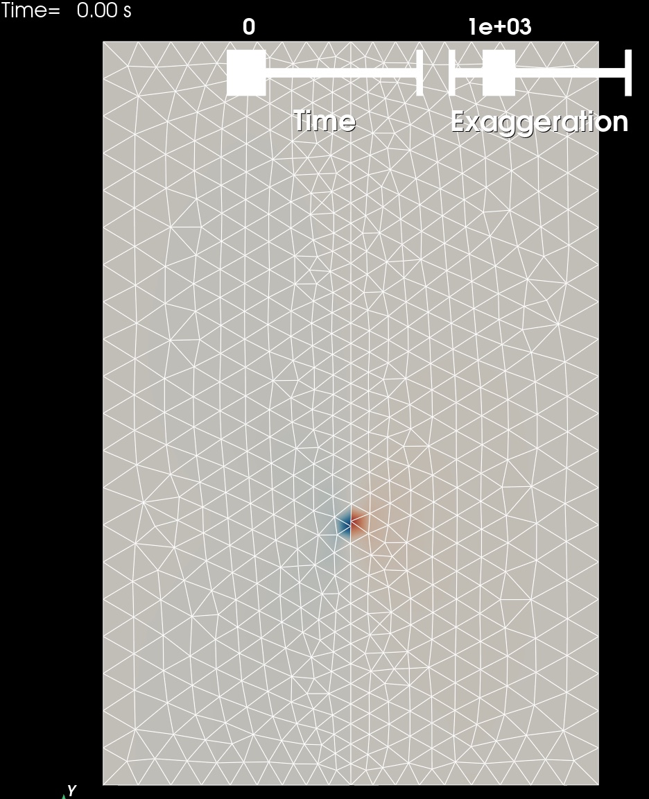
Fig. 70 Solution for Step 4. The colors of the shaded surface indicate the y displacement, and the deformation is exaggerated by a factor of 1000. The time value corresponds to the zero-based index of the slip impulses.