
Step 1: Axial Compression#
This example involves a static simulation that solves for the deformation from axial compression. Fig. 147 shows the boundary conditions on the domain.

Fig. 147 Boundary conditions for axial compression in the x direction with roller boundary conditions on the -y, +y, and -z boundaries.#
Features
Tetrahedral cells
pylith.meshio.MeshIOCubit
pylith.problems.TimeDependent
pylith.meshio.OutputSolnBoundary
pylith.meshio.DataWriterHDF5
pylith.bc.DirichletTimeDependent
pylith.bc.ZeroDB
spatialdata.geocoords.CSGeo
pylith.materials.Elasticity
pylith.materials.IsotropicLinearElasticity
spatialdata.spatialdb.SimpleDB
Static simulation
pylith.materials.IsotropicLinearElasticity
spatialdata.spatialdb.SimpleDB
Simulation parameters#
The parameters specific to this example are in step01_axialdisp.cfg and include:
pylithapp.metadataMetadata for this simulation. Even when the author and version are the same for all simulations in a directory, we prefer to keep that metadata in each simulation file as a reminder to keep it up-to-date for each simulation.pylithappParameters defining where to write the output.pylithapp.problem.bcParameters for describing the boundary conditions that override the defaults.
We override the parameters for the Dirichlet displacement boundary conditions on the -x and +x boundaries.
We replace the ZeroDB spatial database for zero displacement values with a UniformDB to impose axial compression with 2.0 m of displacement on the two boundaries.
For a more efficient solve we use the PETSc default solver options for elasticity in parallel;
for larger simulations these are sometimes more efficient than the defaults for running in serial.
$ pylith step01_axialdisp.cfg mat_elastic.cfg

# The output should look something like the following.
>> /software/pylith-opt/lib/python3.12/site-packages/pylith/apps/PyLithApp.py:77:main
-- pylithapp(info)
-- Running on 1 process(es).
>> /software/pylith-opt/lib/python3.12/site-packages/pylith/meshio/MeshIOObj.py:41:read
-- meshiopetsc(info)
-- Reading finite-element mesh
>> /src/cig/pylith/libsrc/pylith/meshio/MeshIO.cc:74:void pylith::meshio::MeshIO::read(pylith::topology::Mesh*, bool)
-- meshiopetsc(info)
-- Component 'meshiopetsc.reader': Domain bounding box:
    (-400000, 400000)
    (-400000, 400000)
    (-400000, 2017.5)

# -- many lines omitted --
>> /software/pylith-opt/lib/python3.12/site-packages/pylith/problems/Problem.py:250:_printInfo
-- timedependent(info)
-- Scales for nondimensionalization:
    Length scale: 20000*m
    Displacement scale: 1*m
    Time scale: 3.15576e+09*s
    Rigidity scale: 1e+10*m**-1*kg*s**-2
    Temperature scale: 1*K
>> /software/pylith-opt/lib/python3.12/site-packages/pylith/problems/Problem.py:217:initialize
-- timedependent(info)
-- Initializing timedependent problem with quasistatic formulation.
>> /src/cig/pylith/libsrc/pylith/utils/PetscOptions.cc:262:static void pylith::utils::_PetscOptions::write(pythia::journal::info_t&, const char*, const pylith::utils::PetscOptions&)
-- petscoptions(info)
-- Setting PETSc options:
ksp_converged_reason = true
ksp_error_if_not_converged = true
ksp_gmres_restart = 100
ksp_guess_pod_size = 8
ksp_guess_type = pod
ksp_rtol = 1.0e-14
mg_fine_ksp_max_it = 5
pc_type = gamg
snes_atol = 5.0e-7
snes_converged_reason = true
snes_error_if_not_converged = true
snes_monitor = true
snes_rtol = 1.0e-14
ts_error_if_step_fails = true
ts_exact_final_time = matchstep
ts_monitor = true
ts_type = beuler
viewer_hdf5_collective = true
>> /software/pylith-opt/lib/python3.12/site-packages/pylith/problems/TimeDependent.py:145:run
-- timedependent(info)
-- Solving problem.
0 TS dt 0.001 time 0.
    0 SNES Function norm 1.673924902061e+03
      Linear solve converged due to CONVERGED_ATOL iterations 14
    1 SNES Function norm 1.647222821241e-07
    Nonlinear solve converged due to CONVERGED_FNORM_ABS iterations 1
1 TS dt 0.001 time 0.001
>> /software/pylith-opt/lib/python3.12/site-packages/pylith/problems/Problem.py:232:finalize
-- timedependent(info)
-- Finalizing problem.
At the beginning of the output written to the terminal, we see that PyLith is reading the mesh using the MeshIOPetsc reader and that it found the domain to extend from -400 km to +400 km in the x direction, from -400 km to +400 km in the y direction, and from -400 km to +2 km in the z direction.
The output also includes the scales used for nondimensionalization and the default PETSc options.
At the end of the output written to the terminal, we see that the solver advanced the solution 1 time step (static simulation).
The linear solve converged after 14 iterations and the norm of the residual met the absolute convergence tolerance (ksp_atol) .
The nonlinear solve converged in 1 iteration, which we expect because this is a linear problem, and the residual met the absolute convergence tolerance (snes_atol).
$ pylith step01_axialdisp.cfg step01_axialdisp_cubit.cfg mat_elastic.cfg
Visualizing the results#
The output directory contains the simulation output.
Each “observer” writes its own set of files, so the solution over the domain is in one set of files, the boundary condition information is in another set of files, and the material information is in yet another set of files.
The HDF5 (.h5) files contain the mesh geometry and topology information along with the solution fields.
The Xdmf (.xmf) files contain metadata that allow visualization tools like ParaView to know where to find the information in the HDF5 files.
To visualize the data using ParaView or Visit, load the Xdmf files.
In Fig. 148 we use the pylith_viz utility to visualize the x displacement field.
pylith_viz --filename=output/step01_axialdisp-domain.h5 warp_grid --component=x --exaggeration=10000
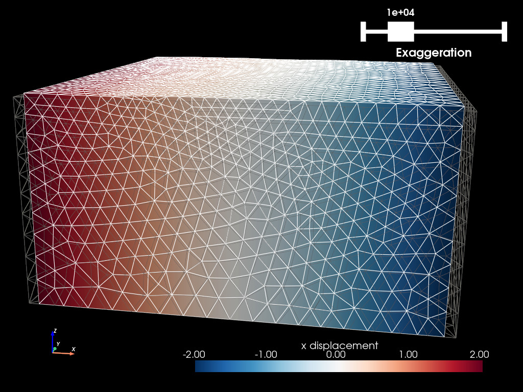
Fig. 148 Solution for Step 1. The colors of the shaded surface indicate the x displacement, and the deformation is exaggerated by a factor of 10,000.#