
Step 1: No faults, no flexure#
Features
Quasi-static problem
triangular cells
LU preconditioner
pylith.materials.Poroelasticity
pylith.meshio.MeshIOPetsc
pylith.problems.TimeDependent
pylith.problems.SolnDispPresTracStrainVelPdotTdot
pylith.problems.InitialConditionDomain
pylith.bc.DirichletTimeDependent
pylith.bc.NeumannTimeDependent
pylith.meshio.DataWriterHDF5
spatialdata.spatialdb.SimpleGridDB
Simulation parameters#
This example uses poroelasticity to model the infiltration of seawater through a slab of oceanic lithosphere. The permeability field is depth dependent, decreasing with depth but does not vary laterally. The lithosphere is not subject to any deformation, but a fluid pressure is applied to the top boundary that is equivalent to the pressure exerted on the seafloor by the water column. This simulates what the hydration state of the oceanic lithosphere is far from any spreading centers, or convergent margins. It also serves as a comparison to see how the hydration state varies for later steps where more complexities are introduced.
Fig. 175 shows the boundary conditions on the domain.
The parameters specific to this example are in step01_no_faults_no_flexure.cfg.

Fig. 175 Boundary and initial conditions for Step 1. We fix the left and the top boundaries with a zero displacement boundary condition, while leaving the right and bottom boundaries unconstrained. We impose a fluid pressure on the +y boundary equal to the weight of the water column to generate fluid flow.#
SimpleGridDB file that does not contain enhanced permeability due to outer rise faults.#[pylithapp.problem]
[pylithapp.problem.materials.slab]
db_auxiliary_field.filename = no_faultzone_permeability.spatialdb
Running the simulation#
$ pylith step01_no_faults_no_flexure.cfg

# The output should look something like the following.
>> software/pylith-debug/lib/python3.12/site-packages/pylith/apps/PyLithApp.py:79:main
-- info (application-flow)
-- Running on 1 process(es).

# -- many lines omitted --
>> src/cig/pylith/libsrc/pylith/problems/TimeDependent.cc:473:void pylith::problems::TimeDependent::solve()
-- info (application-flow)
-- Component 'timedependent.problem': Solving equations.
0 TS dt 8.41536 time -8.41536
    0 SNES Function norm 1.780933174156e+03
      Linear solve converged due to CONVERGED_ATOL iterations 23
    1 SNES Function norm 9.489171115501e-10
    Nonlinear solve converged due to CONVERGED_FNORM_ABS iterations 1
1 TS dt 8.41536 time 0.
    0 SNES Function norm 2.440019354463e-03
      Linear solve converged due to CONVERGED_ATOL iterations 22
    1 SNES Function norm 3.000361522615e-13
    Nonlinear solve converged due to CONVERGED_FNORM_ABS iterations 1

# -- many lines omitted --

50 TS dt 8.41536 time 412.353
    0 SNES Function norm 2.201389334854e-05
      Linear solve converged due to CONVERGED_ATOL iterations 18
    1 SNES Function norm 3.145787316430e-13
    Nonlinear solve converged due to CONVERGED_FNORM_ABS iterations 1
51 TS dt 8.41536 time 420.768
>> software/pylith-debug/lib/python3.12/site-packages/pylith/problems/Problem.py:222:finalize
-- info (application-flow)
-- Finalizing problem.
Visualizing the results#
The output directory contains the simulation output.
Each “observer” writes its own set of files, so the solution over the domain is in one set of files, the boundary condition information is in another set of files, and the material information is in yet another set of files.
The HDF5 (.h5) files contain the mesh geometry and topology information along with the solution fields.
The Xdmf (.xmf) files contain metadata that allow visualization tools like ParaView to know where to find the information in the HDF5 files.
To visualize the data using ParaView or Visit, load the Xdmf files.
In Fig. 176 we use the pylith_viz utility to visualize the porosity field.
pylith_viz --filenames=output/step01_no_faults_no_flexure-slab.h5 warp_grid --field=porosity --exaggeration=1 --hide-edges
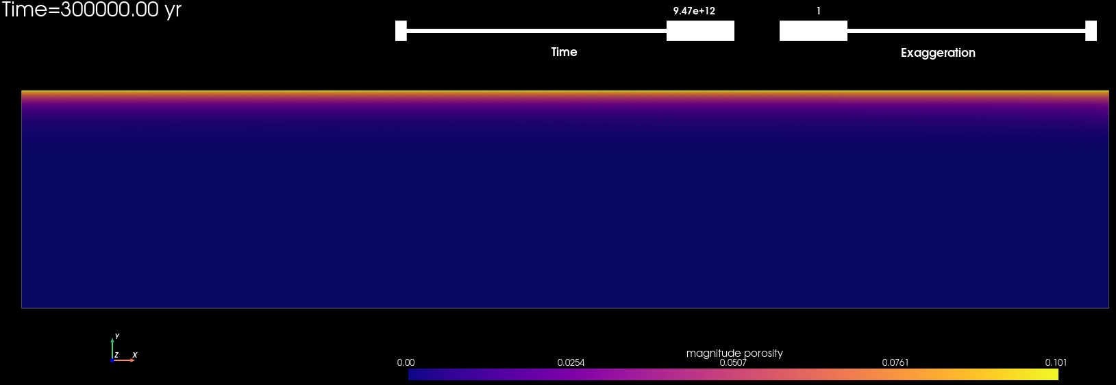
Fig. 176 Porosity field at the end of model run time for Step 1.#