Step 4: Variable Coseismic Slip

Features

• Triangular cells

• pylith.meshio.MeshIOPetsc

• pylith.problems.TimeDependent

• pylith.materials.Elasticity

• pylith.materials.IsotropicLinearElasticity

• pylith.faults.FaultCohesiveKin

• pylith.faults.KinSrcStep

• field split preconditioner

• Schur complement preconditioner

• pylith.bc.DirichletTimeDependent

• spatialdata.spatialdb.UniformDB

• pylith.meshio.OutputSolnBoundary

• pylith.meshio.DataWriterHDF5

• Static simulation

Simulation parameters

We use this example to illustrate prescribing slip that varies along the strike of the fault. This example also serves as a means to generate coseismic displacements at fake GNSS stations. In Step 6 we will use the displacements at these stations along with static Green’s functions computed in Step 5 to invert for the slip on the fault.

We prescribe left-lateral slip that varies along the strike of the fault with fixed displacements on the +x and -x boundaries (Fig. 66), similar to what we had in Step 1. The slip is nonzero over the region -20 km \(\le\) y \(\le\) +20 km with a peak slip of 80 cm at y=-0.5 km (Fig. 68).

This example involves a static simulation that solves for the deformation from prescribed coseismic slip on the fault. Fig. 66 shows the boundary conditions on the domain. The parameters specific to this example are in step04_varslip.cfg.

Fig. 66 Boundary conditions for static coseismic slip. We set the x and y displacement to zero on the +x and -x boundaries and prescribe left-lateral slip that varies along strike.

For greater accuracy in modeling the spatial variation in slip, we refine the mesh by a factor of 2 and use a basis order of 2 for the solution subfields.

Listing 87 Parameters related to increasing the basis order of the solution subfields to 2.

[pylithapp.problem]
defaults.quadrature_order = 2

[pylithapp.problem.solution.subfields]
displacement.basis_order = 2
lagrange_multiplier_fault.basis_order = 2


[pylithapp.problem.materials.elastic_xneg]
derived_subfields.cauchy_strain.basis_order = 1
derived_subfields.cauchy_stress.basis_order = 1

[pylithapp.problem.materials.elastic_xpos]
derived_subfields.cauchy_strain.basis_order = 1
derived_subfields.cauchy_stress.basis_order = 1

We also add output of the solution at fake GNSS stations given in the file gnss_stations.txt. You can use the Python script generate_gnssstations.py to generate a different random set of stations; the default parameters will generate the provided gnss_stations.txt file.

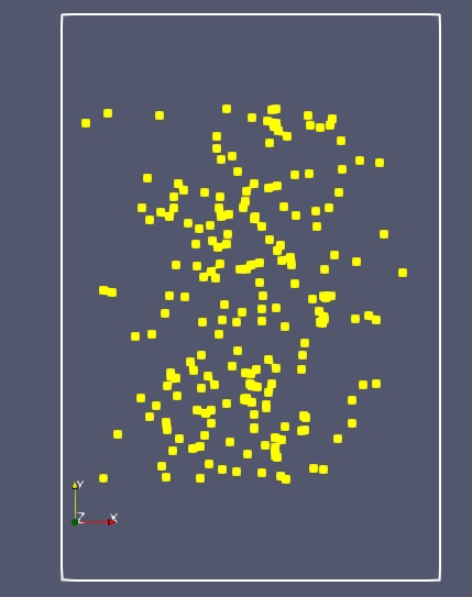
Fig. 67 Location of randomly distributed fake GNSS stations in gnss_stations.txt.

Listing 88 Solution and output parameters for Step 4. We add output of the solution at fake GNSS stations.

[pylithapp.problem]
solution_observers = [domain, top_boundary, bot_boundary, gnss_stations]
solution_observers.gnss_stations = pylith.meshio.OutputSolnPoints

[pylithapp.problem.solution_observers.gnss_stations]
label = gnss_stations
reader.filename = gnss_stations.txt
reader.coordsys.space_dim = 2

Listing 89 Solution and output parameters for Step 4. We add output of the solution at fake GNSS stations.

[pylithapp.problem]
solution_observers = [domain, top_boundary, bot_boundary, gnss_stations]
solution_observers.gnss_stations = pylith.meshio.OutputSolnPoints

[pylithapp.problem.solution_observers.gnss_stations]
label = gnss_stations
reader.filename = gnss_stations.txt
reader.coordsys.space_dim = 2

The earthquake rupture occurs along the central portion of the fault with spatially variable slip.

Fig. 68 Prescribed left-lateral slip that varies along the strike of the fault. A strike of 0 corresponds to y=0.

We use a SimpleGridDB to define the spatial variation in slip.

Listing 90 Prescribed slip parameters for Step 4. We refine the fault mesh by a factor of 8 (3 levels of refinement by a factor of 2) so that the output, which uses a basis order of 1, better captures the discretization of slip, which uses a basis order of 2.

[pylithapp.problem.interfaces.fault]
observers.observer.refine_levels = 3

[pylithapp.problem.interfaces.fault.eq_ruptures.rupture]
db_auxiliary_field = spatialdata.spatialdb.SimpleDB
db_auxiliary_field.description = Fault rupture auxiliary field spatial database
db_auxiliary_field.iohandler.filename = slip_variable.spatialdb
db_auxiliary_field.query_type = linear

Running the simulation

Listing 91 Run Step 4 simulation

$ pylith step04_varslip.cfg

# The output should look something like the following.
 >> /software/unix/py3.12-venv/pylith-debug/lib/python3.12/site-packages/pylith/apps/PyLithApp.py:77:main
 -- pylithapp(info)
 -- Running on 1 process(es).
 >> /software/unix/py3.12-venv/pylith-debug/lib/python3.12/site-packages/pylith/meshio/MeshIOObj.py:38:read
 -- meshiopetsc(info)
 -- Reading finite-element mesh
 >> /src/cig/pylith/libsrc/pylith/meshio/MeshIO.cc:85:void pylith::meshio::MeshIO::read(pylith::topology::Mesh *, const bool)
 -- meshiopetsc(info)
 -- Component 'reader': Domain bounding box:
    (-50000, 50000)
    (-75000, 75000)

# -- many lines omitted --

 >> /software/unix/py3.12-venv/pylith-debug/lib/python3.12/site-packages/pylith/problems/TimeDependent.py:132:run
 -- timedependent(info)
 -- Solving problem.
0 TS dt 0.01 time 0.
    0 SNES Function norm 5.220560316093e-03
      Linear solve converged due to CONVERGED_ATOL iterations 27
    1 SNES Function norm 1.523809186100e-12
    Nonlinear solve converged due to CONVERGED_FNORM_ABS iterations 1
1 TS dt 0.01 time 0.01
 >> /software/unix/py3.12-venv/pylith-debug/lib/python3.12/site-packages/pylith/problems/Problem.py:199:finalize
 -- timedependent(info)
 -- Finalizing problem.

The beginning of the output written to the terminal matches that in our previous simulations. At the end of the output written to the terminal, we see that the solver advanced the solution one time step (static simulation). The linear solve converged after 27 iterations and the norm of the residual met the absolute convergence tolerance (ksp_atol). The nonlinear solve converged in 1 iteration, which we expect because this is a linear problem, and the residual met the absolute convergence tolerance (snes_atol).

Earthquake rupture parameters

We use the pylith_eqinfo utility to compute rupture information, such as earthquake magnitude, seismic moment, seismic potency, and average slip. For 2D simulations, the average slip provides the most useful information. pylith_eqinfo is a Pyre application and you specify parameters using cfg files and the command line. It writes results to a Python script for use in post-processing of simulation results.

The file eqinfoapp.cfg holds the parameters for pylith_eqinfo in this example. By default, pylith_eqinfo extracts information for the final time step in the output file. In order to compute the seismic moment and moment magnitude, we need the shear modulus for the fault. We account for the contrast in rigidity across the fault by using the effective shear modulus from Wu and Chen [2003] and set the shear wave speed to 3.46 km/s.

Listing 92 Run pylith_eqinfo for the Step 4 simulation.

$ pylith_eqinfo

Listing 93 Contents of output/step04_varslip-eqinfo.py generated by pylith_eqinfo. The all object includes earthquake rupture information combined from all of the individual faults.

class RuptureStats(object):
    pass
all = RuptureStats()
all.timestamp = [  3.155760e+07]
all.ruparea = [  6.300870e+04]
all.potency = [  1.306180e+04]
all.moment = [  3.909267e+14]
all.avgslip = [  2.073016e-01]
all.mommag = [  3.694730e+00]
fault = RuptureStats()
fault.timestamp = [  3.155760e+07]
fault.ruparea = [  6.300870e+04]
fault.potency = [  1.306180e+04]
fault.moment = [  3.909267e+14]
fault.avgslip = [  2.073016e-01]
fault.mommag = [  3.694730e+00]

Visualizing the results

In Fig. 69 we use the pylith_viz utility to visualize the y displacement field.

Listing 94 Visualize PyLith output using pylith_viz.

pylith_viz --filename=output/step04_varslip-domain.h5 warp_grid --component=y

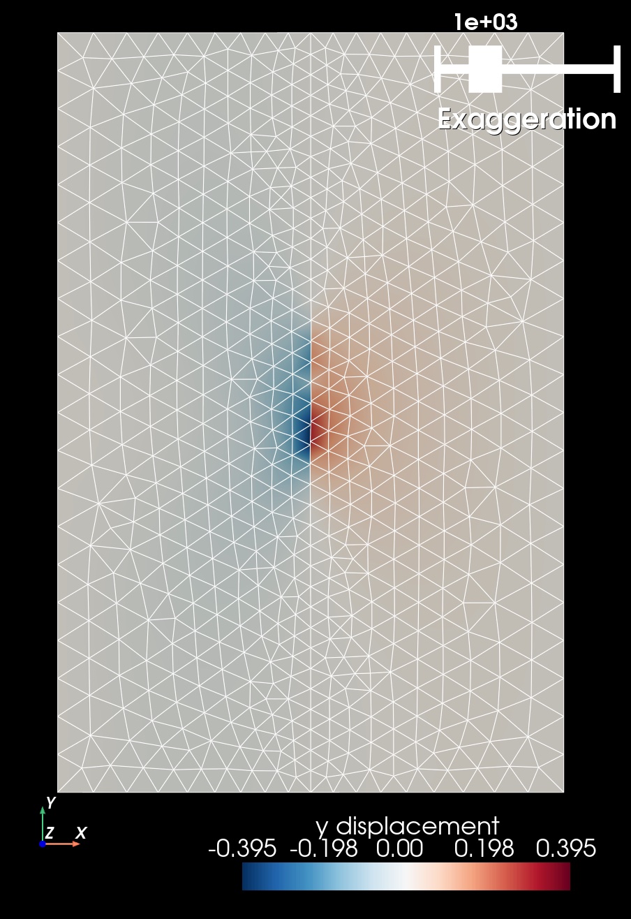
Fig. 69 Solution for Step 4. The colors of the shaded surface indicate the y displacement, and the deformation is exaggerated by a factor of 1000.