
Step 1: Static Coseismic Slip#
Features
Triangular cells
pylith.meshio.MeshIOPetsc
pylith.problems.TimeDependent
pylith.materials.Elasticity
pylith.materials.IsotropicLinearElasticity
pylith.faults.FaultCohesiveKin
pylith.faults.KinSrcStep
field split preconditioner
Schur complement preconditioner
pylith.bc.DirichletTimeDependent
spatialdata.spatialdb.UniformDB
pylith.meshio.OutputSolnBoundary
pylith.meshio.DataWriterHDF5
Static simulation
This example involves a static simulation that solves for the deformation from prescribed coseismic slip on the fault. Fig. 55 shows the boundary conditions on the domain.

Fig. 55 Boundary conditions for static coseismic slip. We set the x and y displacement to zero on the +x and -x boundaries and prescribe 2 meters of right-lateral slip.#
Step 1a: Coarse Mesh#
Note
New in v4.1.0.
We start with a coarse resolution mesh and increase the resolution of the simulation by using uniform refinement or increasing the basis order of the solution fields.
Simulation parameters#
The parameters specific to this example are in step01a_slip.cfg.
[pylithapp.problem.interfaces.fault.eq_ruptures.rupture]
db_auxiliary_field = spatialdata.spatialdb.UniformDB
db_auxiliary_field.description = Fault rupture auxiliary field spatial database
db_auxiliary_field.values = [initiation_time, final_slip_left_lateral, final_slip_opening]
db_auxiliary_field.data = [0.0*s, -2.0*m, 0.0*m]
Running the simulation#
$ pylith step01a_slip.cfg

# The output should look something like the following.
 >> /software/unix/py3.12-venv/pylith-debug/lib/python3.12/site-packages/pylith/apps/PyLithApp.py:77:main
 -- pylithapp(info)
 -- Running on 1 process(es).
 >> /software/unix/py3.12-venv/pylith-debug/lib/python3.12/site-packages/pylith/meshio/MeshIOObj.py:38:read
 -- meshiopetsc(info)
 -- Reading finite-element mesh
 >> /src/cig/pylith/libsrc/pylith/meshio/MeshIO.cc:85:void pylith::meshio::MeshIO::read(pylith::topology::Mesh *, const bool)
 -- meshiopetsc(info)
 -- Component 'reader': Domain bounding box:
    (-50000, 50000)
    (-75000, 75000)
 >> /software/unix/py3.12-venv/pylith-debug/lib/python3.12/site-packages/pylith/faults/FaultCohesiveKin.py:87:preinitialize
 -- faultcohesivekin(info)
 -- Pre-initializing fault 'fault'.
 >> /software/unix/py3.12-venv/pylith-debug/lib/python3.12/site-packages/pylith/problems/Problem.py:116:preinitialize
 -- timedependent(info)
 -- Performing minimal initialization before verifying configuration.
 >> /software/unix/py3.12-venv/pylith-debug/lib/python3.12/site-packages/pylith/problems/Solution.py:39:preinitialize
 -- solution(info)
 -- Performing minimal initialization of solution.
 >> /software/unix/py3.12-venv/pylith-debug/lib/python3.12/site-packages/pylith/materials/RheologyElasticity.py:35:preinitialize
 -- isotropiclinearelasticity(info)
 -- Performing minimal initialization of elasticity rheology 'bulk_rheology'.
 >> /software/unix/py3.12-venv/pylith-debug/lib/python3.12/site-packages/pylith/materials/RheologyElasticity.py:35:preinitialize
 -- isotropiclinearelasticity(info)
 -- Performing minimal initialization of elasticity rheology 'bulk_rheology'.
 >> /software/unix/py3.12-venv/pylith-debug/lib/python3.12/site-packages/pylith/bc/DirichletTimeDependent.py:86:preinitialize
 -- dirichlettimedependent(info)
 -- Performing minimal initialization of time-dependent Dirichlet boundary condition 'bc_xneg'.
 >> /software/unix/py3.12-venv/pylith-debug/lib/python3.12/site-packages/pylith/bc/DirichletTimeDependent.py:86:preinitialize
 -- dirichlettimedependent(info)
 -- Performing minimal initialization of time-dependent Dirichlet boundary condition 'bc_xpos'.
 >> /software/unix/py3.12-venv/pylith-debug/lib/python3.12/site-packages/pylith/faults/FaultCohesiveKin.py:87:preinitialize
 -- faultcohesivekin(info)
 -- Pre-initializing fault 'fault'.
 >> /software/unix/py3.12-venv/pylith-debug/lib/python3.12/site-packages/pylith/problems/Problem.py:174:verifyConfiguration
 -- timedependent(info)
 -- Verifying compatibility of problem configuration.
 >> /software/unix/py3.12-venv/pylith-debug/lib/python3.12/site-packages/pylith/problems/Problem.py:219:_printInfo
 -- timedependent(info)
 -- Scales for nondimensionalization:
    Length scale: 1000*m
    Time scale: 3.15576e+09*s
    Pressure scale: 3e+10*m**-1*kg*s**-2
    Density scale: 2.98765e+23*m**-3*kg
    Temperature scale: 1*K
 >> /software/unix/py3.12-venv/pylith-debug/lib/python3.12/site-packages/pylith/problems/Problem.py:185:initialize
 -- timedependent(info)
 -- Initializing timedependent problem with quasistatic formulation.
 >> /src/cig/pylith/libsrc/pylith/utils/PetscOptions.cc:239:static void pylith::utils::_PetscOptions::write(pythia::journal::info_t &, const char *, const PetscOptions &)
 -- petscoptions(info)
 -- Setting PETSc options:
dm_reorder_section = true
dm_reorder_section_type = cohesive
ksp_atol = 1.0e-12
ksp_converged_reason = true
ksp_error_if_not_converged = true
ksp_guess_pod_size = 8
ksp_guess_type = pod
ksp_rtol = 1.0e-12
mg_fine_pc_type = vpbjacobi
pc_type = gamg
snes_atol = 1.0e-9
snes_converged_reason = true
snes_error_if_not_converged = true
snes_monitor = true
snes_rtol = 1.0e-12
ts_error_if_step_fails = true
ts_monitor = true
ts_type = beuler

 >> /software/unix/py3.12-venv/pylith-debug/lib/python3.12/site-packages/pylith/problems/TimeDependent.py:132:run
 -- timedependent(info)
 -- Solving problem.
0 TS dt 0.01 time 0.
    0 SNES Function norm 4.895713226482e-02
    Linear solve converged due to CONVERGED_ATOL iterations 21
    1 SNES Function norm 1.702759841984e-12
  Nonlinear solve converged due to CONVERGED_FNORM_ABS iterations 1
1 TS dt 0.01 time 0.01
 >> /software/unix/py3.12-venv/pylith-debug/lib/python3.12/site-packages/pylith/problems/Problem.py:199:finalize
 -- timedependent(info)
 -- Finalizing problem.
At the beginning of the output written to the terminal, we see that PyLith is reading the mesh using the MeshIOPetsc reader and that it found the domain to extend from -50,000 m to +50,000 m in the x direction and from -75,000 m to +75,000 m in the y direction.
The scales for nondimensionalization remain the default values for a quasistatic problem.
PyLith detects the presence of a fault based on the Lagrange multiplier for the fault in the solution field and selects appropriate preconditioning options as discussed in PETSc Options.
At the end of the output written to the terminal, we see that the solver advanced the solution one time step (static simulation).
The linear solve converged after 21 iterations and the norm of the residual met the absolute convergence tolerance (ksp_atol) .
The nonlinear solve converged in 1 iteration, which we expect because this is a linear problem, and the residual met the absolute convergence tolerance (snes_atol).
Visualizing the results#
The output directory contains the simulation output.
Each “observer” writes its own set of files, so the solution over the domain is in one set of files, the boundary condition information is in another set of files, and the material information is in yet another set of files.
The HDF5 (.h5) files contain the mesh geometry and topology information along with the solution fields.
The Xdmf (.xmf) files contain metadata that allow visualization tools like ParaView to know where to find the information in the HDF5 files.
To visualize the data using ParaView or Visit, load the Xdmf files.
In Fig. 56 and Fig. 57 we use the pylith_viz utility to visualize the simulation results.
pylith_viz --filename=output/step01a_slip-domain.h5 warp_grid --component=y
pylith_viz --filename=output/step01a_slip-elastic_xneg.h5,output/step01a_slip-elastic_xpos.h5 plot_field --field=cauchy_stress --component=xy
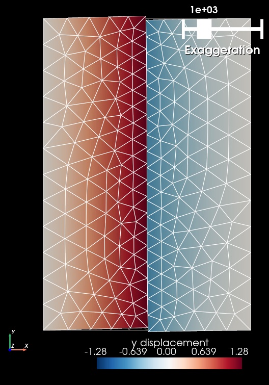
Fig. 56 Solution for Step 1a. The colors of the shaded surface indicate the y displacement, and the deformation is exaggerated by a factor of 1000. The undeformed configuration is shown by the gray wireframe. The contrast in material properties across the faults causes the asymmetry in the y displacement field.#
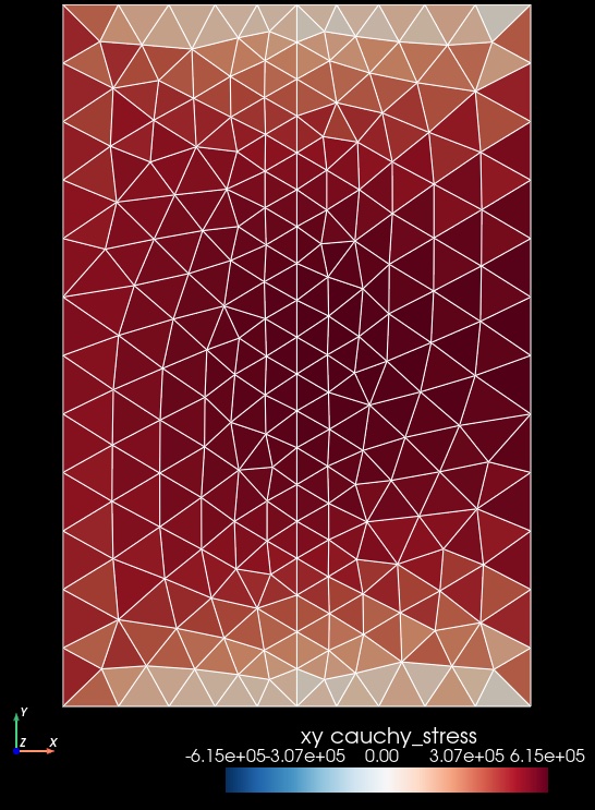
Fig. 57 Cauchy stress component xy for for Step 1a. The colors of the shaded surface indicate the xy stress component. The stress field is uniform within each cell, and the coarse resolution shows a checkerboard pattern near the top and bottom boundaries, which is indicative of poor resolution of the stress field in those regions.#
Step 1a with Cubit Mesh#
Using the Cubit mesh rather than the Gmsh mesh involves two changes:
Use the
MeshIOCubitreader instead of theMeshIOPetscreader and change the filename of the mesh file.Set the
label_valueto 1 for boundary conditions and faults.
We must override the nondefaultlabel_valuesettings inpylithapp.cfgthat were appropriate for our Gmsh reader but are incorrect for the Cubit reader.
The file step01_slip_cubit.cfg provides these changes and updates the names for output.
$ pylith step01_slip_cubit.cfg

# The output should look something like the following.
 >> /software/unix/py3.12-venv/pylith-debug/lib/python3.12/site-packages/pylith/apps/PyLithApp.py:77:main
 -- pylithapp(info)
 -- Running on 1 process(es).
 >> /software/unix/py3.12-venv/pylith-debug/lib/python3.12/site-packages/pylith/meshio/MeshIOObj.py:38:read
 -- meshiocubit(info)
 -- Reading finite-element mesh
 >> /src/cig/pylith/libsrc/pylith/meshio/MeshIOCubit.cc:148:void pylith::meshio::MeshIOCubit::_readVertices(ExodusII &, scalar_array *, int *, int *) const
 -- meshiocubit(info)
 -- Component 'reader': Reading 682 vertices.
 >> /src/cig/pylith/libsrc/pylith/meshio/MeshIOCubit.cc:208:void pylith::meshio::MeshIOCubit::_readCells(ExodusII &, int_array *, int_array *, int *, int *) const
 -- meshiocubit(info)
 -- Component 'reader': Reading 1276 cells in 2 blocks.
 >> /src/cig/pylith/libsrc/pylith/meshio/MeshIOCubit.cc:270:void pylith::meshio::MeshIOCubit::_readGroups(ExodusII &)
 -- meshiocubit(info)
 -- Component 'reader': Found 5 node sets.
 >> /src/cig/pylith/libsrc/pylith/meshio/MeshIOCubit.cc:296:void pylith::meshio::MeshIOCubit::_readGroups(ExodusII &)
 -- meshiocubit(info)
 -- Component 'reader': Reading node set 'fault' with id 10 containing 39 nodes.
 >> /src/cig/pylith/libsrc/pylith/meshio/MeshIOCubit.cc:296:void pylith::meshio::MeshIOCubit::_readGroups(ExodusII &)
 -- meshiocubit(info)
 -- Component 'reader': Reading node set 'boundary_xpos' with id 21 containing 24 nodes.
 >> /src/cig/pylith/libsrc/pylith/meshio/MeshIOCubit.cc:296:void pylith::meshio::MeshIOCubit::_readGroups(ExodusII &)
 -- meshiocubit(info)
 -- Component 'reader': Reading node set 'boundary_xneg' with id 22 containing 24 nodes.
 >> /src/cig/pylith/libsrc/pylith/meshio/MeshIOCubit.cc:296:void pylith::meshio::MeshIOCubit::_readGroups(ExodusII &)
 -- meshiocubit(info)
 -- Component 'reader': Reading node set 'boundary_ypos' with id 23 containing 21 nodes.
 >> /src/cig/pylith/libsrc/pylith/meshio/MeshIOCubit.cc:296:void pylith::meshio::MeshIOCubit::_readGroups(ExodusII &)
 -- meshiocubit(info)
 -- Component 'reader': Reading node set 'boundary_yneg' with id 24 containing 21 nodes.
 >> /src/cig/pylith/libsrc/pylith/meshio/MeshIO.cc:85:void pylith::meshio::MeshIO::read(pylith::topology::Mesh *, const bool)
 -- meshiocubit(info)
 -- Component 'reader': Domain bounding box:
    (-50000, 50000)
    (-75000, 75000)

# -- many lines omitted --

 >> /software/unix/py3.12-venv/pylith-debug/lib/python3.12/site-packages/pylith/problems/TimeDependent.py:132:run
 -- timedependent(info)
 -- Solving problem.
0 TS dt 0.01 time 0.
    0 SNES Function norm 4.834519229177e-02
    Linear solve converged due to CONVERGED_ATOL iterations 22
    1 SNES Function norm 1.188291484607e-12
  Nonlinear solve converged due to CONVERGED_FNORM_ABS iterations 1
1 TS dt 0.01 time 0.01
 >> /software/unix/py3.12-venv/pylith-debug/lib/python3.12/site-packages/pylith/problems/Problem.py:199:finalize
 -- timedependent(info)
 -- Finalizing problem.
The MeshIOCubit reader includes diagnostic information in the journal output related to the sizes of the nodesets and material blocks.
Step 1b: Refined Mesh#
The parameters specific to this example are in step01b_slip.cfg.
Simulation parameters#
In an attempt to better resolve the stress field, we use the same coarse resolution input mesh but add uniform refinement after PyLith reads in the mesh to reduce the discretization size by a factor of 2 in the. During uniform refinement, each triangle is subdivided into four triangles.
[pylithapp.mesh_generator]
refiner = pylith.topology.RefineUniform
Running the simulation#
$ pylith step01b_slip.cfg

# The output will look almost identical to Step 1a.
Visualizing the results#
In Fig. 58 and Fig. 59 we use the pylith_viz utility to visualize the simulation results.
pylith_viz --filename=output/step01b_slip-domain.h5 warp_grid --component=y
pylith_viz --filename=output/step01b_slip-elastic_xneg.h5,output/step01b_slip-elastic_xpos.h5 plot_field --field=cauchy_stress --component=xy
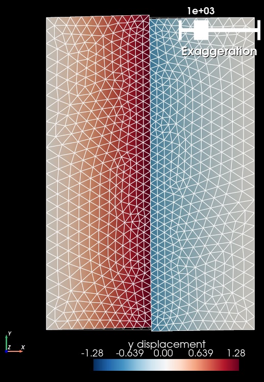
Fig. 58 Solution for Step 1b. The colors of the shaded surface indicate the y displacement, and the deformation is exaggerated by a factor of 1000. The undeformed configuration is shown by the gray wireframe. Uniform refinement reduces the discretization size by a factor of 2.#
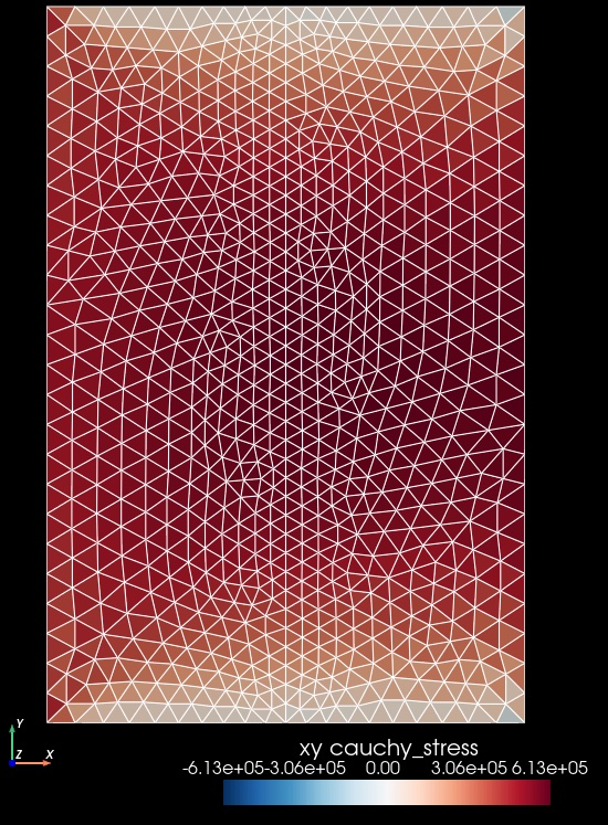
Fig. 59 Cauchy stress component xy for for Step 1b. The colors of the shaded surface indicate the xy stress component. The reduced discretization size results in better resolution of the stress changes near the top and bottom boundaries. However, the stress field is still uniform within each cell, so the checkerboard pattern still persists, albeit with less variation between cells.#
Step 1c: Higher Order Discretization#
The parameters specific to this example are in step01c_slip.cfg.
Simulation parameters#
Increasing the basis order of the solution subfields provides an alternative approach to increasing the resolution of the mesh using uniform refinement.
The accuracy of the stress and strain will be 1 order lower than the basis order of the displacement field. Consequently, we use a basis order of 1 (rather than 0) for the output of the Cauchy stress and strain. We continue to output the solution fields using a basis order of 1, because many visualization tools do not know how to display fields with a basis order of 2. This means the solution subfields in the output are at a reduced resolution compared to the simulation and correspond to projection of each subfield from a basis order of 2 to a basis order of 1.
[pylithapp.problem]
defaults.quadrature_order = 2

[pylithapp.problem.solution.subfields]
displacement.basis_order = 2
lagrange_multiplier_fault.basis_order = 2


[pylithapp.problem.materials.elastic_xneg]
derived_subfields.cauchy_strain.basis_order = 1
derived_subfields.cauchy_stress.basis_order = 1

[pylithapp.problem.materials.elastic_xpos]
derived_subfields.cauchy_strain.basis_order = 1
derived_subfields.cauchy_stress.basis_order = 1
Running the simulation#
$ pylith step01c_slip.cfg

# The output will look almost identical to Steps 1a and 1b.
Visualizing the results#
In Fig. 60 and Fig. 61 we use the pylith_viz utility to visualize the simulation results.
pylith_viz --filename=output/step01c_slip-domain.h5 warp_grid --component=y
pylith_viz --filename=output/step01c_slip-elastic_xneg.h5,output/step01c_slip-elastic_xpos.h5 plot_field --field=cauchy_stress --component=xy
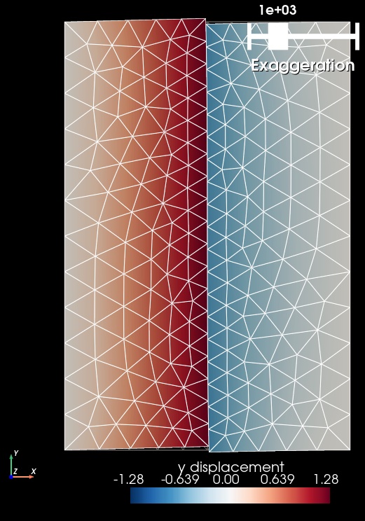
Fig. 60 Solution for Step 1a. The colors of the shaded surface indicate the y displacement, and the deformation is exaggerated by a factor of 1000. The undeformed configuration is shown by the gray wireframe. The displacement field shows little difference from Step 1a.#
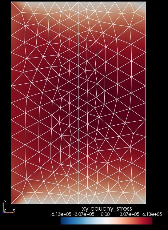
Fig. 61 Cauchy stress component xy for for Step 1a. The colors of the shaded surface indicate the xy stress component. Output with a basis order of 1 shows much better resolution of the shear stress near the top and bottom of the domain with no noticeable checkboard pattern.#
Note
We focus on the displacement field in the subsequent steps in the example, which has sufficient accuracy with a basis order of 1 if we use uniform refinement. Consequently, in the subsequent steps we adopt the uniform refinement parameters that we used in Step 1b.
Key Points#
We can generate a mesh at coarse resolution that captures the geometry and use uniform refinement and high order discretizations of the solution subfields to achieve sufficient resolution.
Using uniform mesh refinement in PyLith requires only two parameter settings: enabling uniform refinement by setting the mesh generator
refinerfacility topylith.topology.RefineUniformand setting the number of levels of refinement.Using higher order discretizations of the solution subfields requires adjusting more parameters that uniform refinement. We adjust the default quadrature order, basis order of the solution fields, and basis order of relevant output fields.
Because uniform mesh refinement requires only a couple of additional parameters, we recommend first using uniform refinement to assess the sensitivity of the results to the discretization size before increasing the basis order of the solution subfields. However, if you know your results are sensitive to the stress field, then we recommend first increasing the basis order.
In some cases, you may find that uniform refinement and higher order discretizations indicate that some portions of the mesh need higher resolution that others, and you might need to adjust the spatial variation of the discretization size in the initial coarse mesh.