Step 4: Earthquake Cycle with Prescribed Slip

This example combines the interseismic deformation from Step 3 and expands on the earthquake ruptures from Step 2. We expand the earthquake ruptures to span the entire along strike length of the top of the slab and also consider earthquake rupture on the splay fault. We use linear Maxwell viscoelastic bulk rheologies in the mantle and deeper part of the slab. Fig. 149 shows the boundary conditions on the domain.

Fig. 149 Boundary conditions for quasi-static interseismic deformation. We prescribe aseismic slip (creep) on the bottom of the slab and the deeper portion of the top of the slab; the shallow portion of the top of the slab remains locked.

Features

• Tetrahedral cells

• pylith.meshio.MeshIOCubit

• pylith.problems.TimeDependent

• pylith.meshio.OutputSolnBoundary

• pylith.meshio.DataWriterHDF5

• pylith.bc.DirichletTimeDependent

• pylith.bc.ZeroDB

• spatialdata.geocoords.CSGeo

• pylith.materials.Elasticity

• pylith.materials.IsotropicLinearElasticity

• pylith.materials.IsotropicLinearMaxwell

• spatialdata.spatialdb.CompositeDB

• spatialdata.spatialdb.SimpleDB

• spatialdata.spatialdb.SimpleGridDB

• pylith.materials.Elasticity

• pylith.materials.IsotropicLinearElasticity

• pylith.materials.IsotropicLinearMaxwell

• spatialdata.spatialdb.CompositeDB

• spatialdata.spatialdb.SimpleDB

• spatialdata.spatialdb.SimpleGridDB

• Quasi-static simulation

• pylith.faults.KinSrcConstRate

• pylith.faults.KinSrcStep

Simulation parameters

The parameters specific to this example are in step04_eqcycle.cfg and include:

• pylithapp.metadata Metadata for this simulation. Even when the author and version are the same for all simulations in a directory, we prefer to keep that metadata in each simulation file as a reminder to keep it up-to-date for each simulation.

• pylithapp Parameters defining where to write the output.

• pylithapp.problem Parameters for the time step information as well as solution field with displacement and Lagrange multiplier subfields.

• pylithapp.interfaces Parameters for the earthquake ruptures and aseismic slip (creep) on the top and bottom of the slab.

• pylithapp.problem.bc Parameters for describing the boundary conditions that override the defaults.

We extend the duration of the simulation to 300 years. We impose two earthquake ruptures on slab interface at t=100 and t=200 years and one earthquake rupture on the splay fault at t=250 years. Now that we have both earthquake rupture and aseismic creep on the top of the slab, we use SimpleDB spatial databases to give depth-dependent, complementary slip. We impose uniform slip on the splay fault using a UniformDB. As in Step 3 we also adjust the nodesets used for the boundary conditions to remove overlap with the slab to allow the slab to move independently. Note that the aseismic slip uses KinSrcConstRate, while the two ruptures use the default KinSrcStep.

Listing 208 Run Step 4 simulation

$ pylith step04_eqcycle.cfg mat_viscoelastic.cfg

# The output should look something like the following.
 >> /software/py38-venv/pylith-opt/lib/python3.8/site-packages/pylith/meshio/MeshIOObj.py:44:read
 -- meshiocubit(info)
 -- Reading finite-element mesh
 >> /pylith/libsrc/pylith/meshio/MeshIOCubit.cc:157:void pylith::meshio::MeshIOCubit::_readVertices(pylith::meshio::ExodusII&,
pylith::scalar_array*, int*, int*) const
 -- meshiocubit(info)
 -- Component 'reader': Reading 24824 vertices.
 >> /pylith/libsrc/pylith/meshio/MeshIOCubit.cc:217:void pylith::meshio::MeshIOCubit::_readCells(pylith::meshio::ExodusII&, pyl
ith::int_array*, pylith::int_array*, int*, int*) const
 -- meshiocubit(info)
 -- Component 'reader': Reading 134381 cells in 4 blocks.

# -- many lines omitted --

 >> /pylith/libsrc/pylith/utils/PetscOptions.cc:235:static void pylith::utils::_PetscOptions::write(pythia::journal::info_t&, const char*, const pylith::utils::PetscOptions&)
 -- petscoptions(info)
 -- Setting PETSc options:
fieldsplit_displacement_ksp_type = preonly
fieldsplit_displacement_mg_levels_ksp_type = richardson
fieldsplit_displacement_mg_levels_pc_type = sor
fieldsplit_displacement_pc_type = gamg
fieldsplit_lagrange_multiplier_fault_ksp_type = preonly
fieldsplit_lagrange_multiplier_fault_mg_levels_ksp_type = richardson
fieldsplit_lagrange_multiplier_fault_mg_levels_pc_type = sor
fieldsplit_lagrange_multiplier_fault_pc_type = gamg
ksp_atol = 1.0e-12
ksp_converged_reason = true
ksp_error_if_not_converged = true
ksp_rtol = 1.0e-12
pc_fieldsplit_schur_factorization_type = lower
pc_fieldsplit_schur_precondition = selfp
pc_fieldsplit_schur_scale = 1.0
pc_fieldsplit_type = schur
pc_type = fieldsplit
pc_use_amat = true
snes_atol = 1.0e-9
snes_converged_reason = true
snes_error_if_not_converged = true
snes_monitor = true
snes_rtol = 1.0e-12
ts_error_if_step_fails = true
ts_monitor = true
ts_type = beuler

# -- many lines omitted --

30 TS dt 0.1 time 2.9
    0 SNES Function norm 8.197330252849e+00
    Linear solve converged due to CONVERGED_ATOL iterations 416
    1 SNES Function norm 4.780619312733e-10
  Nonlinear solve converged due to CONVERGED_FNORM_ABS iterations 1
31 TS dt 0.1 time 3.
 >> /software/unix/py38-venv/pylith-opt/lib/python3.8/site-packages/pylith/problems/Problem.py:201:finalize
 -- timedependent(info)
 -- Finalizing problem.

The beginning of the output is near the same as in Steps 2 and 3. The simulation advances 31 time steps. As in Step 3 each linear solve requires about 400 iterations to converge.

Visualizing the results

In Fig. 150 we use the pylith_viz utility to visualize the x displacement field. You can move the slider or use the p and n keys to change the increment or decrement time.

Listing 209 Visualize PyLith output using pylith_viz.

pylith_viz --filename=output/step04_eqcycle-domain.h5 warp_grid --component=x --exaggeration=5000

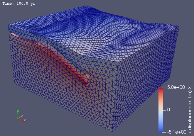
Fig. 150 Solution for Step 4 at t=100 yr. The colors of the shaded surface indicate the x displacement, and the deformation is exaggerated by a factor of 5000.