Step 2: Earthquake Rupture and Postseismic Relaxation

This example involves a quasi-static simulation for coseismic earthquake rupture and postseismic relaxation. We use linear Maxwell viscoelastic bulk rheologies in the mantle and deeper part of the slab. Fig. 145 shows the boundary conditions on the domain.

Fig. 145 Boundary conditions for quasi-static coseismic slip on the subduction interface and postseismic relaxation. We prescribe uniform oblique slip in the center of the subduction interfaces with roller boundary conditions on the lateral sides and bottom of the domain.

Features

• Tetrahedral cells

• pylith.meshio.MeshIOCubit

• pylith.problems.TimeDependent

• pylith.meshio.OutputSolnBoundary

• pylith.meshio.DataWriterHDF5

• pylith.bc.DirichletTimeDependent

• pylith.bc.ZeroDB

• spatialdata.geocoords.CSGeo

• pylith.materials.Elasticity

• pylith.materials.IsotropicLinearElasticity

• pylith.materials.IsotropicLinearMaxwell

• spatialdata.spatialdb.CompositeDB

• spatialdata.spatialdb.SimpleDB

• spatialdata.spatialdb.SimpleGridDB

• pylith.materials.Elasticity

• pylith.materials.IsotropicLinearElasticity

• pylith.materials.IsotropicLinearMaxwell

• spatialdata.spatialdb.CompositeDB

• spatialdata.spatialdb.SimpleDB

• spatialdata.spatialdb.SimpleGridDB

• Quasi-static simulation

• pylith.faults.KinSrcStep

Simulation parameters

The parameters specific to this example are in step02_coseismic.cfg and include:

• pylithapp.metadata Metadata for this simulation. Even when the author and version are the same for all simulations in a directory, we prefer to keep that metadata in each simulation file as a reminder to keep it up-to-date for each simulation.

• pylithapp Parameters defining where to write the output.

• pylithapp.problem Parameters for the time step information as well as solution field with displacement and Lagrange multiplier subfields.

• pylithapp.interfaces Parameters for the earthquake rupture.

We define the duration of the simulation to be 200 years with an initial time step of 10 years. Using the default time stepping algorithm (backward Euler), the time step will remain uniform. Some of the other algorithms adapt the time step to the solution.

For the fault slip, we use the nodesets for the fault and its buried edges corresponding to the central patch of the top of the slab. We set the initiation time to 10 years with the default step time function for the earthquake rupture. We could have also set the origin_time of the earthquake rupture to 10 years and used an initiation_time of 0 years. We impose oblique slip with 1.0 m of right-lateral slip and 4.0 m of reverse slip.

Listing 204 Run Step 2 simulation

$ pylith step02_coseismic.cfg mat_viscoelastic.cfg

# The output should look something like the following.
 >> /software/unix/py3.12-venv/pylith-opt/lib/python3.12/site-packages/pylith/apps/PyLithApp.py:77:main
 -- pylithapp(info)
 -- Running on 1 process(es).
 >> /software/unix/py3.12-venv/pylith-opt/lib/python3.12/site-packages/pylith/meshio/MeshIOObj.py:38:read
 -- meshiocubit(info)
 -- Reading finite-element mesh
 >> /src/cig/pylith/libsrc/pylith/meshio/MeshIOCubit.cc:148:void pylith::meshio::MeshIOCubit::_readVertices(ExodusII &, scalar_array *, int *, int *) const
 -- meshiocubit(info)
 -- Component 'reader': Reading 24824 vertices.
 >> /src/cig/pylith/libsrc/pylith/meshio/MeshIOCubit.cc:208:void pylith::meshio::MeshIOCubit::_readCells(ExodusII &, int_array *, int_array *, int *, int *) const
 -- meshiocubit(info)
 -- Component 'reader': Reading 134381 cells in 4 blocks.
 >> /src/cig/pylith/libsrc/pylith/meshio/MeshIOCubit.cc:270:void pylith::meshio::MeshIOCubit::_readGroups(ExodusII &)
 -- meshiocubit(info)
 -- Component 'reader': Found 22 node sets.


# -- many lines omitted --

 >> /src/cig/pylith/libsrc/pylith/utils/PetscOptions.cc:239:static void pylith::utils::_PetscOptions::write(pythia::journal::info_t &, const char *, const PetscOptions &)
 -- petscoptions(info)
 -- Setting PETSc options:
dm_reorder_section = true
dm_reorder_section_type = cohesive
ksp_atol = 1.0e-12
ksp_converged_reason = true
ksp_error_if_not_converged = true
ksp_guess_pod_size = 8
ksp_guess_type = pod
ksp_rtol = 1.0e-12
mg_fine_pc_type = vpbjacobi
pc_type = gamg
snes_atol = 1.0e-9
snes_converged_reason = true
snes_error_if_not_converged = true
snes_monitor = true
snes_rtol = 1.0e-12
ts_error_if_step_fails = true
ts_monitor = true
ts_type = beuler


# -- many lines omitted --

20 TS dt 0.1 time 1.9
    0 SNES Function norm 8.004499830756e-03
    Linear solve converged due to CONVERGED_ATOL iterations 5
    1 SNES Function norm 1.017500612615e-10
  Nonlinear solve converged due to CONVERGED_FNORM_ABS iterations 1
21 TS dt 0.1 time 2.
 >> /software/unix/py3.12-venv/pylith-opt/lib/python3.12/site-packages/pylith/problems/Problem.py:199:finalize
 -- timedependent(info)
 -- Finalizing problem.

At the beginning of the output written to the terminal, we see that PyLith is reading the mesh using the MeshIOCubit reader. We also see the PETSc solver options, which show use of the variable point-block Jacobi and GAMG (algebriac multigrid) preconditioner settings.

At the end of the output written to the terminal, we see that the solver advanced the solution 21 time steps. The linear solve converged after 5 iterations and the norm of the residual met the absolute convergence tolerance (ksp_atol) . The nonlinear solve converged in 1 iteration, which we expect because this is a linear problem, and the residual met the absolute convergence tolerance (snes_atol).

Visualizing the results

In Fig. 146 we use the pylith_viz utility to visualize the x displacement field. You can move the slider or use the p and n keys to change the increment or decrement time.

Listing 205 Visualize PyLith output using pylith_viz.

pylith_viz --filename=output/step02_coseismic-domain.h5 warp_grid --component=x --exaggeration=10000

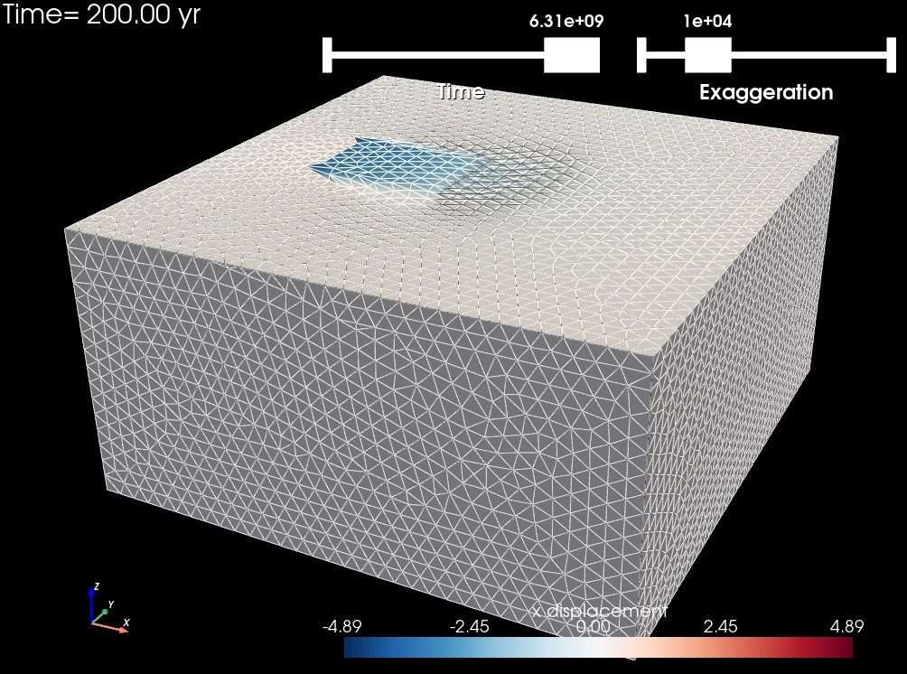
Fig. 146 Solution for Step 2 at t=200 yr. The colors of the shaded surface indicate the x displacement, and the deformation is exaggerated by a factor of 10,000.