Step 7: Slip on Two Faults and Maxwell Viscoelastic Materials#
Features
Triangular cells
pylith.meshio.MeshIOPetsc
pylith.problems.TimeDependent
pylith.bc.DirichletTimeDependent
spatialdata.spatialdb.SimpleDB
spatialdata.spatialdb.ZeroDB
pylith.meshio.OutputSolnBoundary
pylith.meshio.DataWriterHDF5
Quasi-static simulation
pylith.materials.Elasticity
pylith.materials.IsotropicLinearMaxwell
pylith.faults.FaultCohesiveKin
pylith.faults.KinSrcStep
spatialdata.spatialdb.UniformDB
Simulation parameters#
In this example we replace the linear, isotropic elastic bulk rheology in the slab with a linear, isotropic Maxwell viscoelastic rheology.
We also switch from a static simulation to a quasistatic simulation to compute the time-dependent relaxation in the slab.
We use the same boundary conditions as in Step 6.
The parameters specific to this example are in step07_twofaults_maxwell.cfg.
We use a very short relaxation time of 20 years, so we run the simulation for 100 years with a time step of 4 years. We use a starting time of -4 years so that the first time step will advance the solution time to 0 years.
[pylithapp.problem]
initial_dt = 4.0*year
start_time = -4.0*year
end_time = 100.0*year

normalizer.relaxation_time = 20.0*year
[pylithapp.problem.materials]
slab.bulk_rheology = pylith.materials.IsotropicLinearMaxwell

[pylithapp.problem.materials.slab]
db_auxiliary_field = spatialdata.spatialdb.SimpleDB
db_auxiliary_field.description = Maxwell viscoelastic properties
db_auxiliary_field.iohandler.filename = mat_maxwell.spatialdb

bulk_rheology.auxiliary_subfields.maxwell_time.basis_order = 0
Running the simulation#
$ pylith step07_twofaults_maxwell.cfg

# The output should look something like the following.
 >> /software/unix/py39-venv/pylith-debug/lib/python3.9/site-packages/pylith/meshio/MeshIOObj.py:44:read
 -- meshiopetsc(info)
 -- Reading finite-element mesh
 >> /src/cig/pylith/libsrc/pylith/meshio/MeshIO.cc:94:void pylith::meshio::MeshIO::read(pylith::topology::Mesh*)
 -- meshiopetsc(info)
 -- Component 'reader': Domain bounding box:
    (-100000, 100000)
    (-100000, 0)

# -- many lines omitted --

25 TS dt 0.2 time 4.8
    0 SNES Function norm 2.589196279152e-05
    Linear solve converged due to CONVERGED_ATOL iterations 339
    1 SNES Function norm 6.643244443329e-13
  Nonlinear solve converged due to CONVERGED_FNORM_ABS iterations 1
26 TS dt 0.2 time 5.
 >> /software/unix/py39-venv/pylith-debug/lib/python3.9/site-packages/pylith/problems/Problem.py:201:finalize
 -- timedependent(info)
 -- Finalizing problem.
From the end of the output written to the terminal window, we see that the simulation advanced the solution 26 time steps. The PETSc TS display time in the nondimensional units, so a time of 5 corresponds to 100 years.
Visualizing the results#
The output directory contains the simulation output.
Each “observer” writes its own set of files, so the solution over the domain is in one set of files, the boundary condition information is in another set of files, and the material information is in yet another set of files.
The HDF5 (.h5) files contain the mesh geometry and topology information along with the solution fields.
The Xdmf (.xmf) files contain metadata that allow visualization tools like ParaView to know where to find the information in the HDF5 files.
To visualize the data using ParaView or Visit, load the Xdmf files.
In Fig. 83 we use ParaView to visualize the y displacement field using the viz/plot_dispwarp.py Python script.
First, we start ParaView from the examples/reverse-2d directory.
Before running the viz/plot_dispwarp.py Python script as described in ParaView Python Scripts, we set the simulation name in the ParaView Python Shell.
>>> SIM = "step07_twofaults_maxwell"
>>> FIELD_COMPONENT = "X"
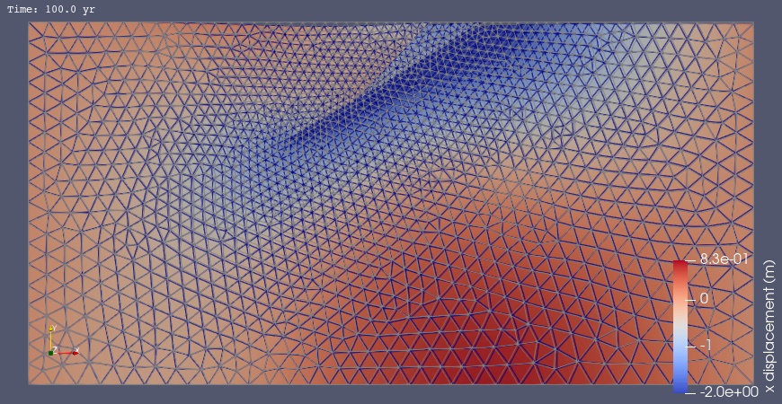
Fig. 83 Solution for Step 7 at t=100 years.
The colors of the shaded surface indicate the magnitude of the x displacement, and the deformation is exaggerated by a factor of 1000.
The undeformed configuration is show by the gray wireframe.
Viscoelastic relaxation results in significant deformation in the slab material.#