Cubit Mesh

Geometry

We construct the geometry by taking a horizontal cross-section of a 3D block. Alternatively, we could have constructed the geometry by building it up from points and curves like we did with Gmsh. Fig. 70 shows the geometry and variables names of the vertices and curves.

Fig. 70 Geometry created in Cubit for generating the finite-element mesh. The names of the verties and curves match the ones we use in the Cubit journal files.

Meshing using Journal Scripts

We use Cubit journal files mesh_tri.jou and mesh_quad.jou to generate triangular and quadrilateral meshes, respectively. Both of these journal files make use of the geometry.jou, gradient.jou, and createbc.jou files for creating the geometry, setting the discretization size, and tagging boundary conditions, faults, and materials, respectively. We use the Cubit graphical user interface to play the Journal files.

We create a brick, extracting a midsurface from it, and then splitting the remaining surface with an extended fault and a splay surface. We then assign names to the surfaces, curves, and important vertices that we use when we specify the mesh sizing information and defining blocks and nodesets.

Important

We use IDless journaling in CUBIT. This allows us to reference objects in a manner that should be independent of the version of CUBIT that is being used. In the journal files, the original command used is typically commented out, and the following command is the equivalent IDless command.

Important

In addition to providing nodesets for the fault and splay, it is also important to provide nodesets defining the buried edges of these two surfaces. In 2D this consists of a single vertex for each surface. This information is required by PyLith to form the corresponding cohesive cells defining fault surfaces.

Note

Examine how we set the discretization size in Gmsh and Cubit. In both cases the discretization size increases at a geometric rate with distance from the main fault. For this simple geometry, it required less than 10 lines of Python code in Gmsh but significantly more lines in Cubit. In Gmsh the code is very general and remains the same even as the domain geometry becomes more complex, whereas in Cubit the number of commands increases quickly as the geometry becomes more complex.

Once you have run either the mesh_tri.jou or mesh_quad.jou journal file to construct the geometry and generate the mesh, you will have a corresponding Exodus-II file (mesh_tri.exo or mesh_quad.exo). These are NetCDF files, and they can be loaded into ParaView. This can be done by either running ParaView and loading the file, or using the script provided in the viz directory. For example, if ParaView is in your path, you can run the following command:

Listing 96 Start paraview and run the viz/plot_mesh.py Python script to view the mesh with triangular cells.

paraview --script=viz/plot_mesh.py

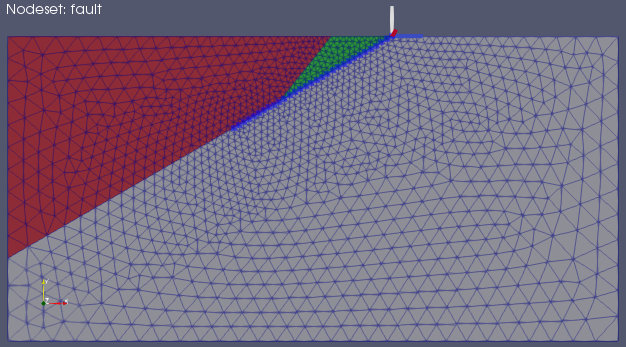
Fig. 71 Finite-element mesh with triangular cells generated by Cubit.

To load the mesh with quadrilateral cells, open the Python Shell in ParaView and set the EXODUS_FILE variable, and then run the viz/plot_mesh.py Python script. See ParaView Python Scripts for more information about running ParaView Python scripts.

Listing 97 Load a different Exodus file generated by Cubit by setting the EXODUS_FILE variable in the ParaView Python Shell.

EXODUS_FILE = "mesh_quad.exo"

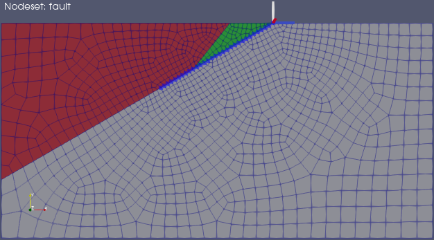
Fig. 72 Finite-element mesh with quadrilateral cells generated by Cubit.