Step 4: Surface Tractions#
Features
Triangular cells
pylith.meshio.MeshIOPetsc
pylith.problems.TimeDependent
pylith.bc.DirichletTimeDependent
spatialdata.spatialdb.SimpleDB
spatialdata.spatialdb.ZeroDB
pylith.meshio.OutputSolnBoundary
pylith.meshio.DataWriterHDF5
Static simulation
pylith.materials.Elasticity
pylith.materials.IsotropicLinearElasticity
pylith.bc.NeumannTimeDependent
Simulation parameters#
This example focuses on loading via surface tractions on the +y boundary.
We apply tractions normal to the boundary with a trapezoidal distribution as shown in Fig. 77
We use the same roller boundary conditions that we used in Steps 1-3.
The parameters specific to this example are in step04_surfload.cfg.

Fig. 77 We add a Neumann (traction) boundary condition on the +y boundary with roller boundary conditions on the lateral sides and bottom of the domain.#
[pylithapp.problem]
bc = [bc_xneg, bc_xpos, bc_yneg, bc_ypos]
bc.bc_ypos = pylith.bc.NeumannTimeDependent

[pylithapp.problem.bc.bc_ypos]
label = boundary_ypos
label_value = 13

db_auxiliary_field = spatialdata.spatialdb.SimpleDB
db_auxiliary_field.description = Neumann BC +y edge
db_auxiliary_field.iohandler.filename = traction_surfload.spatialdb

db_auxiliary_field.query_type = linear

auxiliary_subfields.initial_amplitude.basis_order = 1
Running the simulation#
$ pylith step04_surfload.cfg

# The output should look something like the following.
 >> /software/unix/py39-venv/pylith-debug/lib/python3.9/site-packages/pylith/meshio/MeshIOObj.py:44:read
 -- meshiopetsc(info)
 -- Reading finite-element mesh
 >> /src/cig/pylith/libsrc/pylith/meshio/MeshIO.cc:94:void pylith::meshio::MeshIO::read(pylith::topology::Mesh*)
 -- meshiopetsc(info)
 -- Component 'reader': Domain bounding box:
    (-100000, 100000)
    (-100000, 0)

# -- many lines omitted --

 >> /software/unix/py39-venv/pylith-debug/lib/python3.9/site-packages/pylith/problems/TimeDependent.py:139:run
 -- timedependent(info)
 -- Solving problem.
0 TS dt 0.01 time 0.
    0 SNES Function norm 1.213351093160e-02
    Linear solve converged due to CONVERGED_ATOL iterations 1
    1 SNES Function norm 1.038106792811e-15
  Nonlinear solve converged due to CONVERGED_FNORM_ABS iterations 1
1 TS dt 0.01 time 0.01
 >> /software/unix/py39-venv/pylith-debug/lib/python3.9/site-packages/pylith/problems/Problem.py:201:finalize
 -- timedependent(info)
 -- Finalizing problem.
As expected from the use of the LU preconditioner and linear problem, both the linear and nonlinear solvers converged in 1 iterations.
Visualizing the results#
The output directory contains the simulation output.
Each “observer” writes its own set of files, so the solution over the domain is in one set of files, the boundary condition information is in another set of files, and the material information is in yet another set of files.
The HDF5 (.h5) files contain the mesh geometry and topology information along with the solution fields.
The Xdmf (.xmf) files contain metadata that allow visualization tools like ParaView to know where to find the information in the HDF5 files.
To visualize the data using ParaView or Visit, load the Xdmf files.
In Fig. 78 we use ParaView to visualize the displacement field using the viz/plot_dispwarp.py Python script.
First, we start ParaView from the examples/reverse-2d directory.
Before running the viz/plot_dispwarp.py Python script as described in ParaView Python Scripts, we set the simulation name in the ParaView Python Shell.
>>> SIM = "step04_surfload"
>>> WARP_SCALE = 500
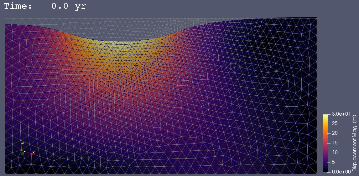
Fig. 78 Solution for Step 4. The colors of the shaded surface indicate the magnitude of the displacement, and the deformation is exaggerated by a factor of 500. The undeformed configuration is show by the gray wireframe.#