Step 2: Shear Displacement

This example corresponds to shear deformation due to Dirichlet (displacement) boundary conditions. We apply Dirichlet (displacement) boundary conditions for the y displacement on the +x (boundary_xpos) and -x (boundary_xneg) boundaries and for the x displacement on the +y (boundary_ypos) and -y (boundary_yneg) boundaries. Fig. 39 shows the boundary conditions on the domain.

Fig. 41 Boundary conditions for shear deformation. We constrain the y displacement on the +x and -x boundaries and the x displacement on the +y and -y boundaries.

Features

• Tetrahedral cells

• pylith.meshio.MeshIOPetsc

• pylith.problems.TimeDependent

• pylith.materials.Elasticity

• pylith.materials.IsotropicLinearElasticity

• spatialdata.spatialdb.UniformDB

• pylith.meshio.OutputSolnBoundary

• pylith.meshio.DataWriterHDF5

• Static simulation

• LU preconditioner

• pylith.bc.DirichletTimeDependent

• spatialdata.spatialdb.SimpleDB

• spatialdata.spatialdb.ZeroDB

Simulation parameters

The parameters specific to this example are in step02_sheardisp.cfg. These include:

• pylithapp.metadata Metadata for this simulation. Even when the author and version are the same for all simulations in a directory, we prefer to keep that metadata in each simulation file as a reminder to keep it up-to-date for each simulation.

• pylithapp Parameters defining where to write the output.

• pylithapp.problem.solution Specify the basis order for the solution fields, in this case the displacement field.

• pylithapp.problem.bc Parameters for the boundary conditions. The displacement field varies along the boundary, so we use a SimpleDB spatial database and the linear query type.

Listing 36 Run Step 2 simulation

$ pylith step02_sheardisp.cfg

# The output should look something like the following.
 >> /software/unix/py39-venv/pylith-debug/lib/python3.9/site-packages/pylith/meshio/MeshIOObj.py:44:read
 -- meshiopetsc(info)
 -- Reading finite-element mesh
 >> /src/cig/pylith/libsrc/pylith/meshio/MeshIO.cc:94:void pylith::meshio::MeshIO::read(topology::Mesh *)
 -- meshiopetsc(info)
 -- Component 'reader': Domain bounding box:
    (-6000, 6000)
    (-6000, 6000)
    (-9000, 0)

# -- many lines omitted --

 >> /software/unix/py39-venv/pylith-debug/lib/python3.9/site-packages/pylith/problems/TimeDependent.py:139:run
 -- timedependent(info)
 -- Solving problem.
0 TS dt 0.01 time 0.
    0 SNES Function norm 1.811215061775e-02 
    Linear solve converged due to CONVERGED_ATOL iterations 1
    1 SNES Function norm 2.330640615892e-17 
  Nonlinear solve converged due to CONVERGED_FNORM_ABS iterations 1
1 TS dt 0.01 time 0.01
 >> /software/unix/py39-venv/pylith-debug/lib/python3.9/site-packages/pylith/problems/Problem.py:201:finalize
 -- timedependent(info)
 -- Finalizing problem.

The output written to the terminal is nearly identical to what we saw for Step 1.

Visualizing the results

In Fig. 42 we use ParaView to visualize the x displacement field using the viz/plot_dispwarp.py Python script. First, we start ParaView from the examples/box-2d directory.

Listing 37 Open ParaView using the command line.

$ PATH_TO_PARAVIEW/paraview

# For macOS, it will be something like
$ /Applications/ParaView-5.10.1.app/Contents/MacOS/paraview

Next, we override the default name of the simulation file with the name of the current simulation.

Listing 38 Set the simulation in the ParaView Python Shell.

>>> SIM = "step02_sheardisp"

Finally, we run the viz/plot_dispwarp.py Python script as described in ParaView Python Scripts.

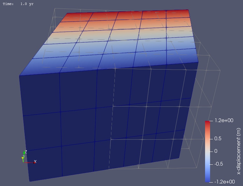
Fig. 42 Solution for Step 2. The colors of the shaded surface indicate the magnitude of the x displacement, and the deformation is exaggerated by a factor of 1000. The undeformed configuration is show by the gray wireframe.