Step 8: Slip on Two Faults and Power-law Viscoelastic Materials

In this example we replace the linear, isotropic Maxwell viscoelastic bulk rheology in the slab in Step 7 with an isotropic powerlaw viscoelastic rheology. The other parameters remain the same as those in Step 6.

Features

• Triangular cells

• pylith.meshio.MeshIOPetsc

• pylith.problems.TimeDependent

• pylith.bc.DirichletTimeDependent

• spatialdata.spatialdb.SimpleDB

• spatialdata.spatialdb.ZeroDB

• pylith.meshio.OutputSolnBoundary

• pylith.meshio.DataWriterHDF5

• Quasistatic simulation

• pylith.materials.Elasticity

• pylith.materials.IsotropicPowerLaw

• pylith.faults.FaultCohesiveKin

• pylith.faults.KinSrcStep

• spatialdata.spatialdb.UniformDB

Simulation parameters

The parameters specific to this example are in step08_twofaults_powerlaw.cfg and include:

• pylithapp.metadata Metadata for this simulation. Even when the author and version are the same for all simulations in a directory, we prefer to keep that metadata in each simulation file as a reminder to keep it up-to-date for each simulation.

• pylithapp Parameters defining where to write the output.

• pylithapp.problem Parameters for the time stepping and solution field with displacement and Lagrange multiplier subfields.

• pylithapp.problem.material Parameters for the linear powerlaw viscoelastic bulk rheology for the slab.

• pylithapp.problem.fault Parameters for prescribed slip on the two faults.

We set the nondimensional time scale (normalizer.relaxation_time) to 5 yearsuse a very short relaxation time of 20 years, so we run the simulation for 100 years with a time step of 4 years. We use a starting time of -4 years so that the first time step will advance the solution time to 0 years.

Important

Both faults contain one end that is buried within the domain. The splay fault ends where it meets the main fault. When PyLith inserts cohesive cells into a mesh with buried edges (in this case a point), we must identify these buried edges so that PyLith properly adjusts the topology along these edges.

For properly topology of the cohesive cells, the main fault must be listed first in the array of faults so that it will be created before the splay fault.

Listing 81 Run Step 8 simulation

$ pylith step08_twofaults_powerlaw.cfg

# The output should look something like the following.
 >> /software/baagaard/py38-venv/pylith-debug/lib/python3.8/site-packages/pylith/meshio/MeshIOObj.py:44:read
 -- meshiopetsc(info)
 -- Reading finite-element mesh
 >> /src/cig/pylith/libsrc/pylith/meshio/MeshIO.cc:94:void pylith::meshio::MeshIO::read(pylith::topology::Mesh*)
 -- meshiopetsc(info)
 -- Component 'reader': Domain bounding box:
    (-100000, 100000)
    (-100000, 0)

# -- many lines omitted --

25 TS dt 0.2 time 4.8
    0 SNES Function norm 5.602869611772e-06 
    Linear solve converged due to CONVERGED_ATOL iterations 262
    1 SNES Function norm 6.656502817834e-08 
    Linear solve converged due to CONVERGED_ATOL iterations 117
    2 SNES Function norm 9.645013365143e-10 
  Nonlinear solve converged due to CONVERGED_FNORM_ABS iterations 2
26 TS dt 0.2 time 5.
 >> /software/baagaard/py38-venv/pylith-debug/lib/python3.8/site-packages/pylith/problems/Problem.py:201:finalize
 -- timedependent(info)
 -- Finalizing problem.

As in Step 7, the simulation advances 26 time steps. With a nonlinear bulk rheology, the nonlinear solver now requires several iterations to converge at each time step.

Visualizing the results

The output directory contains the simulation output. Each “observer” writes its own set of files, so the solution over the domain is in one set of files, the boundary condition information is in another set of files, and the material information is in yet another set of files. The HDF5 (.h5) files contain the mesh geometry and topology information along with the solution fields. The Xdmf (.xmf) files contain metadata that allow visualization tools like ParaView to know where to find the information in the HDF5 files. To visualize the data using ParaView or Visit, load the Xdmf files.

In Fig. 83 we use ParaView to visualize the y displacement field using the viz/plot_dispwarp.py Python script. First, we start ParaView from the examples/reverse-2d directory. Before running the viz/plot_dispwarp.py Python script as described in ParaView Python Scripts, we set the simulation name in the ParaView Python Shell.

Listing 82 Set the simulation and exaggeration in the ParaView Python Shell.

>>> SIM = "step08_twofaults_powerlaw"
>>> FIELD_COMPONENT = "X"

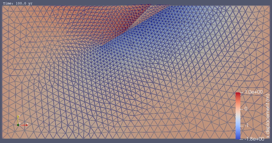
Fig. 83 Solution for Step 8 at t=100 years. The colors of the shaded surface indicate the magnitude of the x displacement, and the deformation is exaggerated by a factor of 1000. The undeformed configuration is show by the gray wireframe. Our parameters for the power-law bulk rheology result in much less viscoelastic relaxation in this case compared to Step 7.