Gmsh Mesh#
Geometry#
We construct the geometry by first creating points, then connecting the points into curves, and finally the curves into surfaces. Fig. 67 shows the geometry and variables names of the vertices and curves.

Fig. 67 Geometry created in Gmsh for generating the finite-element mesh.
We construct curves from points (p1, …, p9) and surfaces from the curves (for example, c_yneg).
The arrows indicate the direction (orientation) of the curves.#
Important
Each curve in Gmsh has a direction (orientation). The direction is from the starting point to the ending point. When connecting curves into surfaces, you must connect the curves in a consistent direction. We connect the curves in a counter-clockwise direction. To reverse the direction of a curve, use the negative tag.
Meshing using Python Script#
We use the Python script generate_gmsh.py to create the geometry and generate the mesh.
The script is structured identically to the one we used in examples/strikeslip-2d.
We create a class App that implements the functionality missing in gmsh_utils.GenerateMesh.
We must implement the create_geometry(), mark(), and generate_mesh() methods that are abstract in the GenerateMesh base class.
The main difference is that the geometry is slightly more complex, and we calculate the location of the points on the fault using trigonometry.
We use the Gmsh MeshSize options to define a discretization size that grows slowly at a geometric rate with distance from the main fault.
# Generate a mesh with triangular cells and save it to `mesh_tri.msh` (default filename).
$ ./generate_gmsh.py --write

# Save as above but start the Gmsh graphical interface after saving the mesh.
$ ./generate_gmsh.py --write --gui

# Create only the geometry and start the Gmsh graphical interface.
$ ./generate_gmsh.py --geometry --gui

# Show available command line arguments.
$ ./generate_gmsh.py --help
By default the Python script will generate a finite-element mesh with triangular cells and save it to the file mesh_tri.msh.
You can view the mesh using Gmsh either by using the --gui command line argument when you generate the mesh or running Gmsh from the command line and opening the file.
gmsh -open mesh_tri.msh
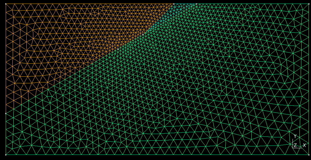
Fig. 68 Finite-element mesh with triangular cells generated by Gmsh.#