Step 6: Slip on Two Faults and Elastic Materials#
In this example we add coseismic slip on the splay fault. We specify 2 meters of reverse slip on the main fault and 1 meter of reverse slip on the splay fault. Fig. 80 shows the boundary conditions on the domain.

Fig. 80 Boundary conditions for static coseismic slip on both the main and splay faults. We prescribe 2 meters of reverse slip on the main fault with 1 meter of reverse slip on the splay fauult. We use roller boundary conditions on the lateral sides and bottom of the domain.#
Features
Triangular cells
pylith.meshio.MeshIOPetsc
pylith.problems.TimeDependent
pylith.bc.DirichletTimeDependent
spatialdata.spatialdb.SimpleDB
spatialdata.spatialdb.ZeroDB
pylith.meshio.OutputSolnBoundary
pylith.meshio.DataWriterHDF5
Static simulation
pylith.materials.Elasticity
pylith.materials.IsotropicLinearElasticity
pylith.faults.FaultCohesiveKin
pylith.faults.KinSrcStep
spatialdata.spatialdb.UniformDB
Simulation parameters#
The parameters specific to this example are in step06_twofaults-elastic.cfg and include:
pylithapp.metadataMetadata for this simulation. Even when the author and version are the same for all simulations in a directory, we prefer to keep that metadata in each simulation file as a reminder to keep it up-to-date for each simulation.pylithappParameters defining where to write the output.pylithapp.problemParameters for the solution field with displacement and Lagrange multiplier subfields.pylithapp.problem.faultParameters for prescribed slip on the two faults.pylithapp.petscAdjustment to the default PETSc solver options.
Important
In 2D simulations slip is specified in terms of opening and left-lateral components. This provides a consistent, unique sense of slip that is independent of the fault orientation. For our geometry in this example, right lateral slip corresponds to reverse slip on both of the dipping faults.
Important
Both faults contain one end that is buried within the domain. The splay fault ends where it meets the main fault. When PyLith inserts cohesive cells into a mesh with buried edges (in this case a point), we must identify these buried edges so that PyLith properly adjusts the topology along these edges.
For properly topology of the cohesive cells, the main fault must be listed first in the array of faults so that it will be created before the splay fault.
$ pylith step06_twofaults_elastic.cfg

# The output should look something like the following.
 >> /software/baagaard/py38-venv/pylith-debug/lib/python3.8/site-packages/pylith/meshio/MeshIOObj.py:44:read
 -- meshiopetsc(info)
 -- Reading finite-element mesh
 >> /src/cig/pylith/libsrc/pylith/meshio/MeshIO.cc:94:void pylith::meshio::MeshIO::read(pylith::topology::Mesh*)
 -- meshiopetsc(info)
 -- Component 'reader': Domain bounding box:
    (-100000, 100000)
    (-100000, 0)

# -- many lines omitted --

 >> /software/unix/py39-venv/pylith-debug/lib/python3.9/site-packages/pylith/problems/TimeDependent.py:139:run
 -- timedependent(info)
 -- Solving problem.
0 TS dt 0.01 time 0.
    0 SNES Function norm 2.225574998436e-02
    Linear solve converged due to CONVERGED_ATOL iterations 415
    1 SNES Function norm 8.564274482242e-13
  Nonlinear solve converged due to CONVERGED_FNORM_ABS iterations 1
1 TS dt 0.01 time 0.01
 >> /software/unix/py39-venv/pylith-debug/lib/python3.9/site-packages/pylith/problems/Problem.py:201:finalize
 -- timedependent(info)
 -- Finalizing problem.
From the end of the output written to the terminal window, we see that the linear solver converged in 415 iterations and met the absolute convergence tolerance (ksp_atol).
As we expect for this linear problem, the nonlinear solver converged in 1 iteration.
Visualizing the results#
The output directory contains the simulation output.
Each “observer” writes its own set of files, so the solution over the domain is in one set of files, the boundary condition information is in another set of files, and the material information is in yet another set of files.
The HDF5 (.h5) files contain the mesh geometry and topology information along with the solution fields.
The Xdmf (.xmf) files contain metadata that allow visualization tools like ParaView to know where to find the information in the HDF5 files.
To visualize the data using ParaView or Visit, load the Xdmf files.
In Fig. 81 we use ParaView to visualize the y displacement field using the viz/plot_dispwarp.py Python script.
First, we start ParaView from the examples/reverse-2d directory.
Before running the viz/plot_dispwarp.py Python script as described in ParaView Python Scripts, we set the simulation name in the ParaView Python Shell.
>>> SIM = "step06_twofaults_elastic"
>>> FIELD_COMPONENT = "X"
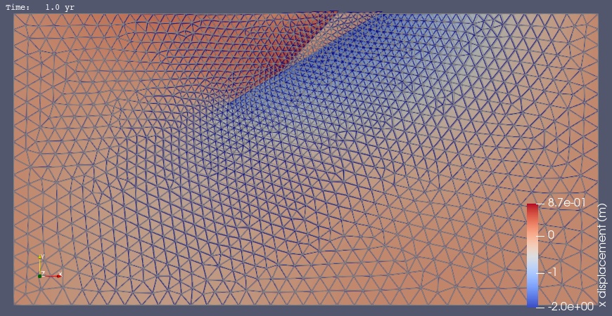
Fig. 81 Solution for Step 6. The colors of the shaded surface indicate the magnitude of the x displacement, and the deformation is exaggerated by a factor of 1000. The undeformed configuration is show by the gray wireframe.#