Adding New Governing Equations and/or Bulk Rheologies

Overview

There are four basic tasks for adding new physics in the form of a governing equation:

1. Select the fields for the solution. This will control the form of the partial differential equation and the terms in the residuals and Jacobians.

2. Derive the pointwise functions for the residuals and Jacobians. Determine flags that will be used to indicate which terms to include.

3. Determine which parameters in the pointwise functions could vary in space as well as any state variables. We bundle all state variables and spatially varying parameters into a field called the auxiliary field. Each material has a separate auxiliary field.

4. Parameters that are spatially uniform are treated separately from the parameters in the auxiliary field.

Material is responsible for the terms in the governing equations associated with the domain (i.e., volume integrals in a 3D domain and surface integrals in a 2D domain). A separate object implements the bulk rheology for a specific governing equation. Fig. 144 shows the objects used to implement multiple rheologies for the elasticity equation: an isotropic, linear elastic rheology for incompressible elasticity, and an isotropic, linear elastic rheology for poroelasticity. The Elasticity object describes the physics for the elasticity equation, including the pointwise functions and flags for turning on optional terms (such as inertia) in the governing equation, and RheologyElasticity defines the interface for bulk elastic rheologies.

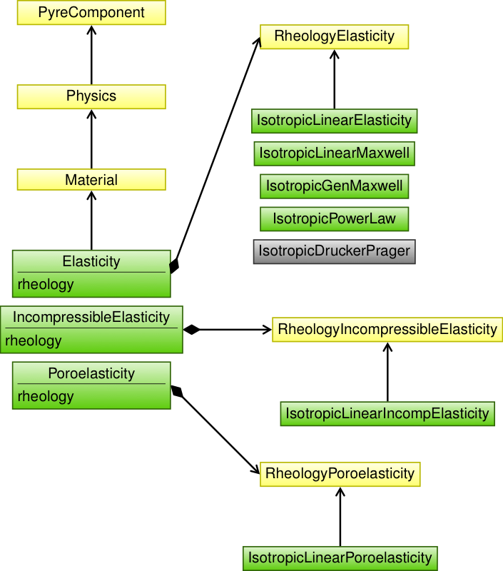
Fig. 144 Class diagram for the implementation of governing equations and bulk rheologies. Each governing equation implementation inherits from the abstract Material class and bulk rheologies inherit from the abstract rheology class specific to that governing equation.

Python

• Define solution subfields.

  • All subfields in the solution field are SolutionSubfield objects (see Fig. 145). PyLith already includes several solution subfields:

    • SubfieldDisplacement Displacement vector field.

    • SubfieldVelocity Velocity vector field.

    • SubfieldLagrangeFault Lagrange multiplier field for fault constraints.

    • SubfieldPressure Fluid pressure or mean stress scalar field.

    • SubfieldTemperature Temperature scalar field.

  • PyLith includes solution field containers with predefined subfields:

    • SolnDisp Solution composed of a displacement field.

    • SolnDispVel Solution composed of displacement and velocity fields.

    • SolnDispPres Solution composed of displacement and mean stress (pressure) fields.

    • SolnDispLagrange Solution composed of displacement and Lagrange multiplier fields.

    • SolnDispPresLagrange Solution composed of displacement, mean stress (pressure), and Lagrange multiplier subfields.

    • SolnDispVelLagrange Solution composed of displacement, velocity, and Lagrange multiplier subfields.

• Define auxiliary subfields.

  The auxiliary subfields for a governing equation are defined as facilities in a Pyre Component. For example, the ones for Elasticity are in AuxFieldsElasticity. The order of the subfields is defined not by the order they are listed in the Pyre component, but by the order they are added to the auxiliary field in the C++ object. The auxiliary subfields bulk rheologies are defined in the same way.

  Important

  A single auxiliary field will be created for each material; it contains the auxiliary subfields from both the governing equation and the bulk rheology.

• Flags to turn on/off terms in governing equation.

  For the elasticity equation, we sometimes do not include body forces or inertial terms in our simulations. Rather than implement these cases as separate materials, we simply include flags in the material to turn these terms on/off. The flags are implemented as Pyre properties in our material component.

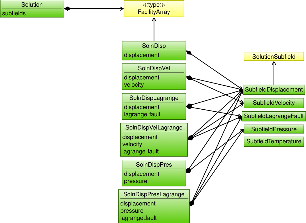
Fig. 145 Class diagram for the solution field, solution subfields, and pre-defined containers of solution subfields.

C++

• Define auxiliary subfields.

  We build the auxiliary field using classes derived from pylith::feassemble::AuxiliaryFactory. The method corresponding to each subfield specifies the name of the subfield, its components, and scale for nondimensionalizing. We generally create a single auxiliary factory object for each governing equation, but not each bulk constitutive model, because constitutive models for the same governing equation often have many of the same subfields. For example, most of our bulk constitutive models for the elasticity contain density, bulk modulus, and shear modulus auxiliary subfields.

  Important

  Within the concrete implementation of the material and bulk rheology objects, we add the subfields to the auxiliary field. The order in which they are added determines the order they will be in the auxiliary field. You will need to use know this order when you implement the pointwise functions. See Fig. 146 for more information on the layout of the auxiliary field.

• Implement the pointwise functions.

  The pointwise functions for the residuals, Jacobians, and projections follow nearly identical interfaces. In most cases you should implement the terms in the governing equation in 3D with 2D plane strain using the more general 3D version. While this is slightly less efficient, it results in less code to maintain.

• Set the pointwise functions.

  We set the pointwise functions for the RHS and LHS residuals and Jacobians, taking into consideration which optional terms of the governing equation have been selected by the user.

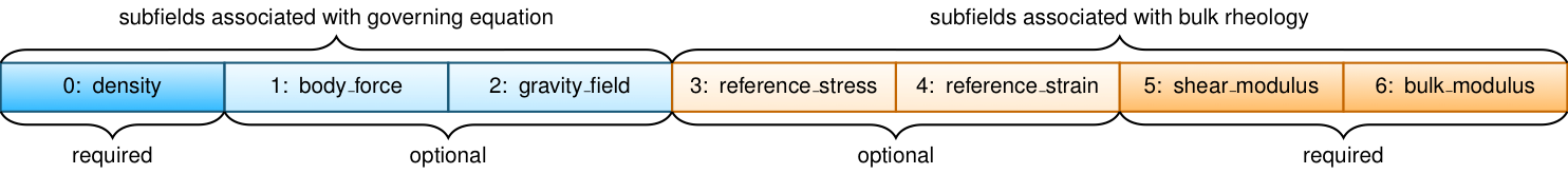
Fig. 146 Layout of material auxiliary subfields. The subfields include those for both the governing equation and the bulk rheology. The required subfields are at the ends with the optionalfields in the middle. This allows the same pointwise functions to be used for some cases with and without the optional subfields.