
Step 7: Generation of Green’s Functions and Slow Slip Inversion#
In this example we compute the static Green’s function for prescribed slip impulses on the central portion of the subduction interface. We then use the responses to perform a simple geodetic inversion of the slip from Step 6. We divide generating Green’s functions into two sub-problems:
Step 7a: Left-lateral slip component
Step 7b: Reverse slip component
Although PyLith can generate the two components in one simulation, we often prefer to speed up the process by running simulations for each of the components simultaneously using multiple processes on a cluster.
Fig. 157 shows the boundary conditions on the domain.

Fig. 157 Boundary conditions for Green’s function generation. We apply left-lateral (Step 7a) and reverse (Step 7b) slip impulses on a patch within the subduction interface with roller boundary conditions on the lateral sides and bottom of the domain.#
Features
Tetrahedral cells
pylith.meshio.MeshIOCubit
pylith.problems.TimeDependent
pylith.meshio.OutputSolnBoundary
pylith.meshio.DataWriterHDF5
pylith.bc.DirichletTimeDependent
pylith.bc.ZeroDB
spatialdata.geocoords.CSGeo
pylith.materials.Elasticity
pylith.materials.IsotropicLinearElasticity
spatialdata.spatialdb.SimpleDB
“Green’s functions”
pylith.problems.GreensFns
pylith.meshio.OutputSolnPoints
pylith.faults.FaultCohesiveImpulses
spatialdata.spatialdb.UniformDB
spatialdata.geocoords.CSGeo
Simulation parameters#
The parameters specific to this example are in step07a_leftlateral.cfg and step07b_reverse.cfg and include:
pylithapp.metadataMetadata for this simulation. Even when the author and version are the same for all simulations in a directory, we prefer to keep that metadata in each simulation file as a reminder to keep it up-to-date for each simulation.pylithappParameters defining where to write the output. We also change the problem type topylith.problems.GreensFns.pylithapp.problemParameters for the time step information as well as solution field with displacement and Lagrange multiplier subfields.pylithapp.interfacesParameters for the slip impulses applied on the top of the slab.
For Green’s functions we use the FaultCohesiveImpulses kinematic source to prescribe slip impulses for left-lateral (Step 7a – impulse_dof = [1]) and reverse (Step 7b – impulse_dof = [2]) slip directions. As for Step 6, we use OutputSolnPoints to output the solution at fake CGNSS stations.
$ pylith step07a_leftlateral.cfg mat_elastic.cfg
$ pylith step07b_reverse.cfg mat_elastic.cfg

# The output should look something like the following.
 >> /home/baagaard/software/micromamba/envs/pylith-opt/lib/python3.12/site-packages/pylith/apps/PyLithApp.py:77:main
 -- pylithapp(info)
 -- Running on 1 process(es).
 >> /home/baagaard/software/micromamba/envs/pylith-opt/lib/python3.12/site-packages/pylith/meshio/MeshIOObj.py:41:read
 -- meshiopetsc(info)
 -- Reading finite-element mesh
 >> /home/baagaard/src/cig/pylith/libsrc/pylith/meshio/MeshIO.cc:74:void pylith::meshio::MeshIO::read(pylith::topology::Mesh*, bool)
 -- meshiopetsc(info)
 -- Component 'meshiopetsc.reader': Domain bounding box:
    (-400000, 400000)
    (-400000, 400000)
    (-400000, 2017.5)

# -- many lines omitted --

 >> /home/baagaard/software/micromamba/envs/pylith-opt/lib/python3.12/site-packages/pylith/problems/GreensFns.py:105:run
 -- greensfns(info)
 -- Solving problem.
 >> /home/baagaard/src/cig/pylith/libsrc/pylith/problems/GreensFns.cc:321:void pylith::problems::GreensFns::solve()
 -- greensfns(info)
 -- Component 'greensfns.problem': Computing Green's function 1 of 96.
  0 SNES Function norm 5.684788384324e-02
    Linear solve converged due to CONVERGED_ATOL iterations 11
  1 SNES Function norm 1.157087800256e-08
  Nonlinear solve converged due to CONVERGED_ITS iterations 1

# -- many lines omitted --

 >> /home/baagaard/src/cig/pylith/libsrc/pylith/problems/GreensFns.cc:321:void pylith::problems::GreensFns::solve()
 -- greensfns(info)
 -- Component 'greensfns.problem': Computing Green's function 96 of 96.
  0 SNES Function norm 6.580456779117e-02
    Linear solve converged due to CONVERGED_ATOL iterations 10
  1 SNES Function norm 6.832632664165e-09
  Nonlinear solve converged due to CONVERGED_ITS iterations 1
 >> /home/baagaard/software/micromamba/envs/pylith-opt/lib/python3.12/site-packages/pylith/problems/Problem.py:232:finalize
 -- greensfns(info)
 -- Finalizing problem.
WARNING! There are options you set that were not used!
WARNING! could be spelling mistake, etc!
There are 4 unused database options. They are:
Option left: name:-ts_error_if_step_fails (no value) source: code
Option left: name:-ts_exact_final_time value: matchstep source: code
Option left: name:-ts_monitor (no value) source: code
Option left: name:-ts_type value: beuler source: code
The beginning of the output is nearly the same as in several previous examples. In this case, however, rather than stepping through time, we are stepping through impulse numbers. In each simulation, there are 96 impulses applied on the fault. Because we are not time stepping, we do not use all of the default PETSc options.
$ pylith step07a_leftlateral.cfg step07a_leftlateral_cubit.cfg mat_elastic.cfg
$ pylith step07b_reverse.cfg step07b_reverse_subit.cfg mat_elastic.cfg
Visualizing the results#
In Fig. 158 we use the pylith_viz utility to visualize the slip for the impulses on the fault surface.
You can move the slider or use the p and n keys to increment or decrement the slip impulse (shown as time).
pylith_viz --filename=output/step07a_leftlateral-fault_slabtop.h5 plot_field --field=slip
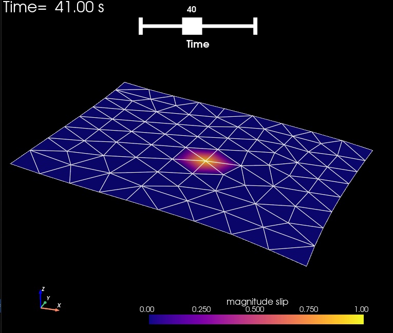
Fig. 158 Distribution of left-lateral fault slip for slip impulse 41 (time corresponds to the zero-based index) for Step 7a. The colors of the shaded surface indicate the magnitude of the slip.#
Performing a simple inversion#
To perform our simulated inversion, we first postprocess the displacement results from Step 6.
We do this using the generate_synthetic_gnssdisp.py Python script, which in turn reads the parameters from the generate_synthetic_gnssdisp.cfg file:
$ ./generate_synthetic_gnssdisp.py
This script will produce the files cgnss_synthetic_displacement.txt, which is used in the inversion.
Once these have been created (and both sets of Green’s functions have been generated), we can perform a simple inversion using the invert_slip.py script, which in turn reads the inversion parameters from invert_slip.cfg.
$ ./invert_slip.py
The Python script performs a simple weighted generalized least-squares inversion, with penalty values applied to the deviation of the solution from the a priori value (zero, in this case).
The slip inversion will produce several files in the output directory:
step07-inversion-summary.txtA summary of the model residuals for each penalty parameter.step07-inversion-displacement.h5The predicted site displacements for different penalty parameters.step07-inversion-slip.h5The predicted fault slip for different penalty parameters.
Note that the inversion produces a .xmf file for each of the HDF5 files.
We provide a Matplotlib Python script to visualize the data misfit for various penalty parameters:
$ viz/plot_inversion_misfit.py
Fig. 159 shows the data residual versus the penalty residual, showing very clearly the ‘corner’ of the L-curve.
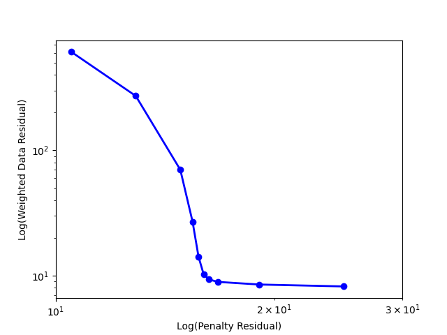
Fig. 159 Data residual versus penalty residual for inversion from Step 7.#