
Step 7: Slip on Two Faults and Maxwell Viscoelastic Materials#
Features
Triangular cells
pylith.meshio.MeshIOPetsc
pylith.problems.TimeDependent
pylith.bc.DirichletTimeDependent
spatialdata.spatialdb.SimpleDB
spatialdata.spatialdb.ZeroDB
pylith.meshio.OutputSolnBoundary
pylith.meshio.DataWriterHDF5
Quasi-static simulation
pylith.materials.Elasticity
pylith.materials.IsotropicLinearMaxwell
pylith.faults.FaultCohesiveKin
pylith.faults.KinSrcStep
spatialdata.spatialdb.UniformDB
Simulation parameters#
In this example we replace the linear, isotropic elastic bulk rheology in the slab with a linear, isotropic Maxwell viscoelastic rheology.
We use the same boundary conditions as in Step 6 but reduce the time step to resolve the viscoelastic relaxation.
The parameters specific to this example are in step07_twofaults_maxwell.cfg.
We use a very short relaxation time of 20 years, so we run the simulation for 100 years with a time step of 4 years. We use a starting time of -4 years so that the first time step will advance the solution time to 0 years.
[pylithapp.problem]
initial_dt = 4.0*year
start_time = -4.0*year
end_time = 100.0*year

scales.relaxation_time = 20.0*year
The uniform slip creates a large stress concentration at the end of the fault. We improve the resolution by using uniform global refinement and discretizing the displacement and Lagrange multiplier fields with a basis order of 2.
[pylithapp.mesh_generator]
refiner = pylith.topology.RefineUniform

[pylithapp.problem]
solution = pylith.problems.SolnDispLagrange
defaults.quadrature_order = 2

[pylithapp.problem.solution.subfields]
displacement.basis_order = 2
lagrange_multiplier_fault.basis_order = 2
[pylithapp.problem.materials]
slab.bulk_rheology = pylith.materials.IsotropicLinearMaxwell

[pylithapp.problem.materials.slab]
db_auxiliary_field = spatialdata.spatialdb.SimpleDB
db_auxiliary_field.description = Maxwell viscoelastic properties
db_auxiliary_field.iohandler.filename = mat_maxwell.spatialdb

bulk_rheology.auxiliary_subfields.maxwell_time.basis_order = 0
Running the simulation#
$ pylith step07_twofaults_maxwell.cfg

# The output should look something like the following.
 >> software/pylith-debug/lib/python3.12/site-packages/pylith/apps/PyLithApp.py:79:main
 -- info (application-flow)
 -- Running on 1 process(es).

# -- many lines omitted --

25 TS dt 0.2 time 4.8
    0 SNES Function norm 3.491930818111e-01
      Linear solve converged due to CONVERGED_ATOL iterations 12
    1 SNES Function norm 6.649621549079e-08
    Nonlinear solve converged due to CONVERGED_FNORM_ABS iterations 1
26 TS dt 0.2 time 5.
 >> software/pylith-debug/lib/python3.12/site-packages/pylith/problems/Problem.py:222:finalize
 -- info (application-flow)
 -- Finalizing problem.
From the end of the output written to the terminal window, we see that the simulation advanced the solution 26 time steps. The PETSc TS display time in the nondimensional units, so a time of 5 corresponds to 100 years.
Visualizing the results#
In Fig. 109 we use the pylith_viz utility to visualize the x displacement field.
You can move the slider or use the p and n keys to change the increment or decrement time.
pylith_viz --filename=output/step07_twofaults_maxwell-domain.h5 warp_grid --component=x
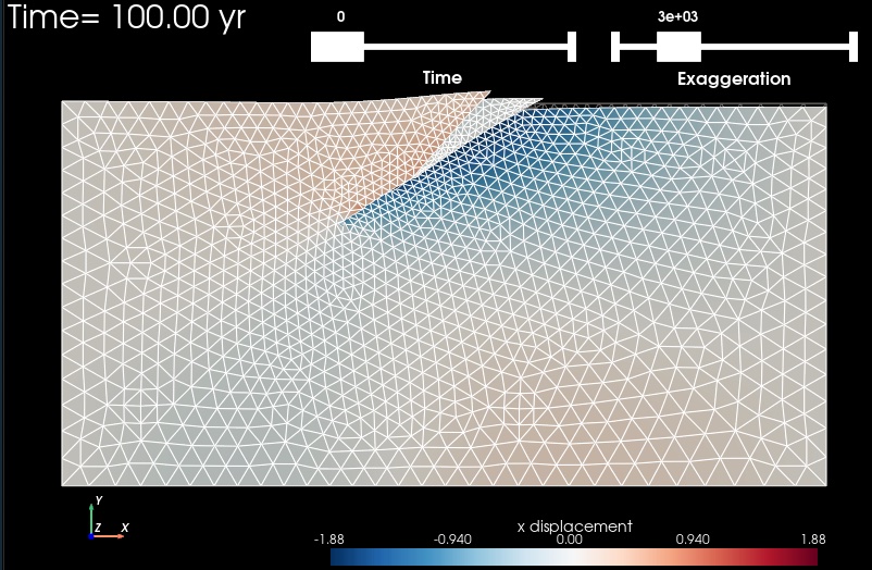
Fig. 109 Solution for Step 7 at t=100 years.
The colors of the shaded surface indicate the x displacement, and the deformation is exaggerated by a factor of 1000.
The undeformed configuration is shown by the gray wireframe.
Viscoelastic relaxation results in significant deformation in the slab material.#
Step 7b: Adaptive Time Stepping#
In Step 7b we demonstrate the use adaptive time stepping. We start with an initial time step of 0.2 years and let the adaptive time stepping algorithm increase the time step as the rate of deformation decreases.
$ pylith step07_twofaults_maxwell.cfg step07b_twofaults_maxwell.cfg

# The output should look something like the following.
 >> software/pylith-debug/lib/python3.12/site-packages/pylith/apps/PyLithApp.py:80:main
 -- info (application-flow)
 -- Running on 1 process(es).

# -- many lines omitted --

 >> src/cig/pylith/libsrc/pylith/problems/TimeDependent.cc:473:void pylith::problems::TimeDependent::solve()
 -- info (application-flow)
 -- Component 'timedependent.problem': Solving equations.
0 TS dt 0.01 time -0.01
    0 SNES Function norm 9.786738657687e+00
      Linear solve converged due to CONVERGED_ATOL iterations 21
    1 SNES Function norm 4.181718260419e-08
    Nonlinear solve converged due to CONVERGED_FNORM_ABS iterations 1
  TSAdapt basic beuler 0: step   0 accepted t=-0.01      + 1.000e-02 dt=1.000e-02
1 TS dt 0.01 time 0.
    0 SNES Function norm 6.800013826439e-02
      Linear solve converged due to CONVERGED_ATOL iterations 15
    1 SNES Function norm 4.941010511485e-08
    Nonlinear solve converged due to CONVERGED_FNORM_ABS iterations 1
  TSAdapt basic beuler 0: step   1 rejected t=0          + 1.000e-02 dt=1.495e-03  wlte= 1.79  wltea=   -1 wlter=   -1
    0 SNES Function norm 3.573809583653e-02
      Linear solve converged due to CONVERGED_ATOL iterations 13
    1 SNES Function norm 3.795363345199e-08
    Nonlinear solve converged due to CONVERGED_FNORM_ABS iterations 1
  TSAdapt basic beuler 0: step   1 accepted t=0          + 1.495e-03 dt=1.041e-03  wlte=0.0824  wltea=   -1 wlter=   -1

# -- many lines omitted --

30 TS dt 0.363756 time 4.63624
    0 SNES Function norm 5.855825329812e-01
      Linear solve converged due to CONVERGED_ATOL iterations 17
    1 SNES Function norm 7.186563774310e-08
    Nonlinear solve converged due to CONVERGED_FNORM_ABS iterations 1
  TSAdapt basic beuler 0: step  30 accepted t=4.63624    + 3.638e-01 dt=3.432e-01  wlte=0.0449  wltea=   -1 wlter=   -1
31 TS dt 0.343229 time 5.
 >> software/pylith-debug/lib/python3.12/site-packages/pylith/problems/Problem.py:222:finalize
 -- info (application-flow)
 -- Finalizing problem.
With smaller time steps following the two earthquakes, this simulation takes 5 more time steps than Step 7 with uniform time steps. For simulations covering longer periods of time or a single earthquake, the adaptive time stepping usually results in substantially fewer time steps.
./plot_compare.py --step=7

Fig. 110 Displacement and shear stress time histories for Step 7 and 7b at a location in the viscoelastic slab below the bottom ends of the main fault and splay fault. The backward Euler time stepping algorithm does a poor job of resolving the rapid deformation following the sudden application of coseismic slip, resulting in some oscillations in the deformation in Step 7b which uses adaptive time stepping.#