Step 2: Quasistatic Interseismic Deformation

Features

• Triangular cells

• field split preconditioner

• Schur complement

• pylith.meshio.MeshIOPetsc

• pylith.problems.TimeDependent

• pylith.materials.Elasticity

• pylith.materials.IsotropicLinearElasticity

• pylith.meshio.OutputSolnBoundary

• pylith.meshio.DataWriterHDF5

• Static simulation

• pylith.faults.FaultCohesiveKin

• pylith.bc.DirichletTimeDependent

• spatialdata.spatialdb.SimpleDB

• spatialdata.spatialdb.UniformDB

• pylith.faults.KinSrcConstRate

• pylith.bc.ZeroDB

Simulation parameters

In this example we simulate the interseismic deformation associated with the oceanic crust subducting beneath the continental crust and into the mantle. We prescribe steady aseismic slip of 8 cm/yr along the interfaces between the oceanic crust and mantle with the interface between the oceanic crust and continental crust locked as shown in Fig. 136. The parameters specific to this example are in step02_interseismic.cfg.

Fig. 136 Boundary conditions for quasistatic simulation for interseismic deformation. We prescribe constant creep on the top and bottom of the subduction slab, except for the portion of the subduction interface where we imposed coseismic slip in Step 1. We lock (zero creep) that part of the interface.

The simulation spans 150 years with an initial time step of 5 years.

Listing 193 Time stepping parameters for Step 2.

[pylithapp.timedependent]
initial_dt = 5.0*year
start_time = -5.0*year
end_time = 150.0*year

We create an array with 2 faults, one for the top of the slab and one for the bottom of the slab. We use the constant slip rate kinematic source model with a uniform slip rate on the bottom of the slab and a slip rate that varies with depth on the top of the slab.

Listing 194 Prescribed slip parameters for Step 2.

[pylithapp.problem]
interfaces = [fault_slabtop, fault_slabbot]

[pylithapp.problem.interfaces.fault_slabtop]
label = fault_slabtop
label_value = 21
edge = fault_slabtop_edge
edge_value = 31

observers.observer.data_fields = [slip, traction_change]

[pylithapp.problem.interfaces.fault_slabtop.eq_ruptures]
rupture = pylith.faults.KinSrcConstRate

[pylithapp.problem.interfaces.fault_slabtop.eq_ruptures.rupture]
db_auxiliary_field = spatialdata.spatialdb.SimpleDB
db_auxiliary_field.description = Fault rupture auxiliary field spatial database
db_auxiliary_field.iohandler.filename = fault_slabtop_creep.spatialdb
db_auxiliary_field.query_type = linear


[pylithapp.problem.interfaces.fault_slabbot]
label = fault_slabbot
label_value = 22
edge = fault_slabbot_edge
edge_value = 32

observers.observer.data_fields = [slip, traction_change]

[pylithapp.problem.interfaces.fault_slabbot.eq_ruptures]
rupture = pylith.faults.KinSrcConstRate

[pylithapp.problem.interfaces.fault_slabbot.eq_ruptures.rupture]
db_auxiliary_field = spatialdata.spatialdb.UniformDB
db_auxiliary_field.description = Fault rupture auxiliary field spatial database
db_auxiliary_field.values = [initiation_time, slip_rate_left_lateral, slip_rate_opening]
db_auxiliary_field.data = [0.0*year, 8.0*cm/year, 0.0*cm/year]

We adjust the Dirichlet (displacement) boundary conditions on the lateral edges and bottom of the domain by pinning only the portions of the boundaries that are mantle and continental crust and not oceanic crust.

Listing 195 We use only 3 Dirichlet boundary conditions to allow the slab to move freely on the boundaries.

[pylithapp.problem]
bc = [bc_east_mantle, bc_west, bc_bottom]

Running the simulation

Listing 196 Run Step 2 simulation

$ pylith step02_interseismic.cfg

# The output should look something like the following.
 >> /software/unix/py3.12-venv/pylith-debug/lib/python3.12/site-packages/pylith/apps/PyLithApp.py:77:main
 -- pylithapp(info)
 -- Running on 1 process(es).
 >> /software/unix/py3.12-venv/pylith-debug/lib/python3.12/site-packages/pylith/meshio/MeshIOObj.py:38:read
 -- meshiopetsc(info)
 -- Reading finite-element mesh
 >> /src/cig/pylith/libsrc/pylith/meshio/MeshIO.cc:85:void pylith::meshio::MeshIO::read(pylith::topology::Mesh *, const bool)
 -- meshiopetsc(info)
 -- Component 'reader': Domain bounding box:
    (-600000, 600000)
    (-600000, 399.651)

# -- many lines omitted --

30 TS dt 0.05 time 1.45
    0 SNES Function norm 5.747931631477e-02
    Linear solve converged due to CONVERGED_ATOL iterations 4
    1 SNES Function norm 5.115112326356e-12
  Nonlinear solve converged due to CONVERGED_FNORM_ABS iterations 1
31 TS dt 0.05 time 1.5
 >> /software/unix/py3.12-venv/pylith-debug/lib/python3.12/site-packages/pylith/problems/Problem.py:199:finalize
 -- timedependent(info)
 -- Finalizing problem.

The beginning of the output written to the terminal is identical to that from Step 1. At the end of the output, we see that the simulation advanced the solution 31 time steps. Remember that the PETSc TS monitor shows the nondimensionalized time and time step values.

Visualizing the results

In Fig. 137 we use the pylith_viz utility to visualize the x displacement field. You can move the slider or use the p and n keys to change the increment or decrement time.

Listing 197 Visualize PyLith output using pylith_viz.

pylith_viz --filename=output/step02_interseismic-domain.h5 warp_grid --component=x

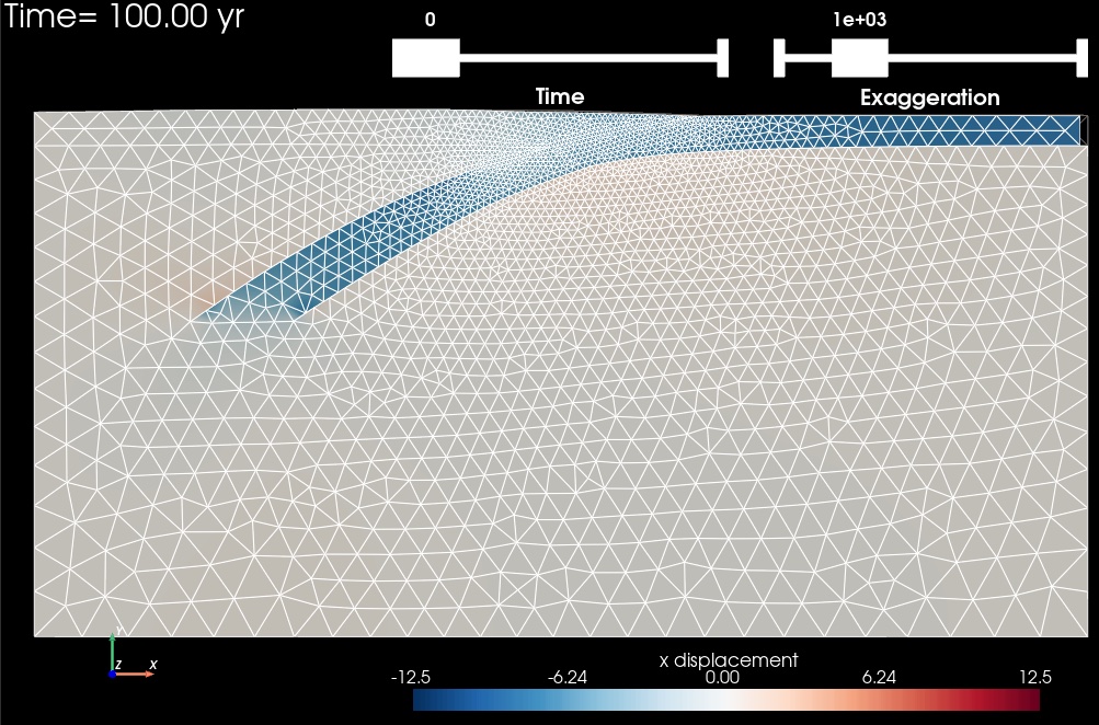
Fig. 137 Solution for Step 2 at t=100 yr. The colors of the shaded surface indicate the x displacement, and the deformation is exaggerated by a factor of 1000.