
Step 4: Shear Displacement and Initial Conditions#
Features
Quadrilateral cells
pylith.meshio.MeshIOAscii
pylith.problems.TimeDependent
pylith.materials.Elasticity
pylith.materials.IsotropicLinearElasticity
spatialdata.spatialdb.UniformDB
pylith.meshio.DataWriterHDF5
Static simulation
LU preconditioner
pylith.problems.InitialConditionDomain
pylith.bc.DirichletTimeDependent
spatialdata.spatialdb.SimpleDB
spatialdata.spatialdb.SimpleGridDB
Simulation parameters#
In this example we demonstrate the use of initial conditions for the boundary value problem in Step 2. We set the displacement field over the domain to the analytical solution as an initial condition.
The parameters specific to this example are in step04_sheardispic.cfg.
The only difference with respect to Step 2 is the addition of the initial condition.
From our boundary conditions we can see that the analytical solution to our boundary value problem is \(\vec{u}(x,y)=(ay,ax)\).
Because we are specifying the displacement field over the domain, we use the SimpleGridDB, which specifies the values on a logically rectangular grid aligned with the coordinate axes.
The grid layout of the values allows queries for values at points to be much more efficient than a SimpleDB which can have points at arbitrary locations.
[pylithapp.problem]
ic = [domain]
ic.domain = pylith.problems.InitialConditionDomain

[pylithapp.problem.ic.domain]
db = spatialdata.spatialdb.SimpleGridDB
db.description = Initial conditions over domain
db.filename = sheardisp_ic.spatialdb
Running the simulation#
$ pylith step04_sheardispic.cfg

# The output should look something like the following.
 >> /software/unix/py39-venv/pylith-debug/lib/python3.9/site-packages/pylith/meshio/MeshIOObj.py:44:read
 -- meshioascii(info)
 -- Reading finite-element mesh
 >> /src/cig/pylith/libsrc/pylith/meshio/MeshIO.cc:94:void pylith::meshio::MeshIO::read(topology::Mesh *)
 -- meshioascii(info)
 -- Component 'reader': Domain bounding box:
    (-6000, 6000)
    (-16000, -0)

# -- many lines omitted --

 >> /software/unix/py39-venv/pylith-debug/lib/python3.9/site-packages/pylith/problems/TimeDependent.py:139:run
 -- timedependent(info)
 -- Solving problem.
0 TS dt 0.01 time 0.
    0 SNES Function norm 4.968438524050e-19
  Nonlinear solve converged due to CONVERGED_FNORM_ABS iterations 0
1 TS dt 0.01 time 0.01
 >> /software/unix/py39-venv/pylith-debug/lib/python3.9/site-packages/pylith/problems/Problem.py:201:finalize
 -- timedependent(info)
 -- Finalizing problem.
WARNING! There are options you set that were not used!
WARNING! could be spelling mistake, etc!
There is one unused database option. It is:
Option left: name:-ksp_converged_reason (no value)
By design we set the initial condition so that it satisfies the elasticity equation. As a result, the first nonlinear solver residual evaluation meets the convergence criteria. The linear solver is not used; this is why PETSc reports an unused option at the end of the simulation.
Visualizing the results#
In Fig. 32 we use the pylith_viz utility to visualize the x displacement field.
pylith_viz --filenames=output/step04_sheardispic-domain.h5 warp_grid --component=x
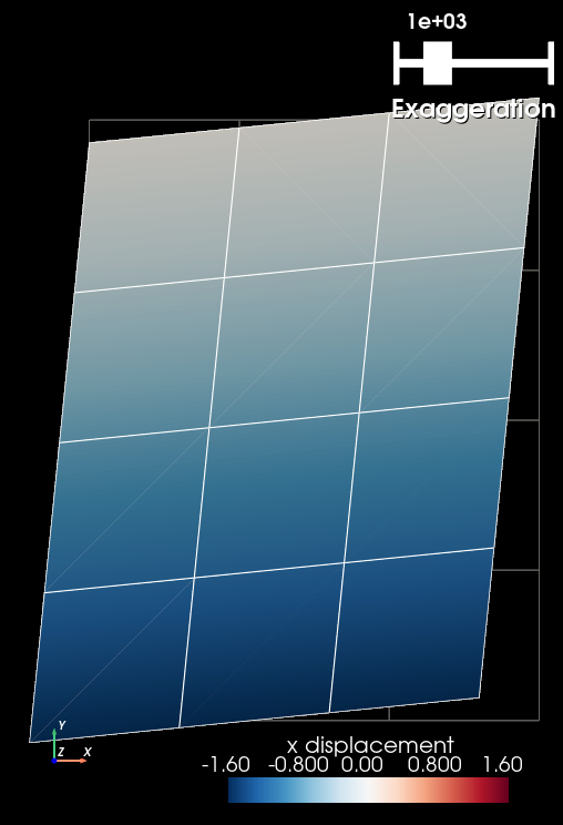
Fig. 32 Solution for Step 4. The colors of the shaded surface indicate the x displacement, and the deformation is exaggerated by a factor of 1000. The undeformed configuration is shown by the gray wireframe. THe solution matches the one in Step 2.#