Cubit Mesh

We use Cubit to generate the finite-element mesh. Due to its size, we do not include the finite-element mesh in the PyLith source or binary distributions. See the instructions in the input/README.md file for how to download the mesh.

Setup

We use contours of the Cascadia Subduction Zone from Slab v1.0 [Hayes et al., 2012] for the geometry of the subduction interface. To make use of these contours from within Cubit, we use a Python script (utils/generate_surfjou.py) to read the contours file and create a Cubit journal file (scratch/cubit_create_surfs.jou) that adds additional contours west of the trench and then constructs the top and bottom surfaces of the slab. The Python script also constructs a splay fault by copying a contour to a depth below the slab and above the ground surface.

Tip

We define the coordinate systems we use in the simulations in the Python script utils/coordsys.py to make it easier to convert to and from various georeference coordinate systems in the pre- and post-processing. PyLith will automatically convert among compatible coordinate systems during the simulation.

Listing 143 Generate generate_surfs.jou

# Make sure you are in the `subduction-3d` directory and then run the Python
# script to generate the journal file `scratch/cubit_create_surfs.jou`.
$ ./utils/generate_surfjou.py

Meshing using Journal Scripts

The next step is to use Cubit to run the scratch/cubit_create_surfs.jou journal file to generate the spline surfaces for the slab and splay fault and save them as ACIS surfaces.

Important

The Cubit journal files name objects and then later reference them by name. When objects are cut, a suffix of @LETTER is appended to the original name (for example, domain becomes domain and domain@A). However, which one retains the original name and which ones gets the suffix is ambiguous. In general, the names are consistent across versions of Cubit with the same version of the underlying ACIS library. As a result, you may need to update the ids in the references to previously named objects that have been split (for example domain@A may need to be changed to domain@B, etc) in order to account for differences in how your version of Cubit has named split objects.

Currently we discretize the domain using a uniform, coarse resolution of 25 km. This allows the simulations to run relatively quickly and fit on a laptop. In a real research problem, we would tailor the resolution to match the length scales we want to capture and use a finer resolution. We provide journal files for both a mesh with tetrahedral cells (cubit_tet.jou) and a mesh with hexahedral cells (cubit_hex.jou). In the following examples, we will focus exclusively on the mesh with tetrahedral cells because the mesh with hexahedral cells contains cells that are significantly distorted; this illustrates how it is often difficult to generate high quality meshes with hexahedral cells for domains with complex 3D geometry.

After you generate the ACIS surface files, run the cubit_tet.jou journal file to construct the geometry, and generate the mesh. In the end you will have an Exodus-II file mesh_tet.exo, which is a NetCDF file, in the input directory. You can load this file into ParaView.

Tip

We recommend carefully examining the cubit_geometry.jou journal file to understand how we assemble the 3D slab and cut the rectangular domain into pieces.

Visualizing the Mesh

The Exodus-II file input/mesh_tet.exo can be viewed with ParaView. We provide the Python script viz/plot_mesh.py to visualize the nodesets and the mesh quality using the condition number metric. As in our other Python scripts for ParaView (see ParaView Python Scripts for a discussion of how to use Python ParaView scripts), you can override the default parameters by setting appropriate values in the Python shell (if running within the ParaView GUI) or from the command line (if running the script directly outside the GUI). When viewing the nodesets, the animation controls allow stepping through the nodesets. When viewing the mesh quality, only the cells with the given quality metric above some threshold (poorer quality) are shown. The default quality metric is condition number and the default threshold is 2.0.

To visualize the mesh, start ParaView. Within the ParaView GUI Python shell (Tools\(\rightarrow\)Python Shell), we override the EXODUS_FILE and SHOW_QUALITY parameters.

Listing 144 ParaView Python shell

# Import the os module so we can get access to the HOME environment variable.
>>> import os
>>> HOME = os.environ["HOME"]
# You may need to adjust the next line, depending on where you installed PyLith.
>>> EXODUS_FILE = os.path.join(HOME,"pylith","examples","subduction-3d","input","mesh_tet.exo")
# Turn off display of the mesh quality (show only the nodesets).
>>> SHOW_QUALITY = False

We then click on the Run Script button and navigate to the examples/subduction-3d/viz directory and select plot_mesh.py.

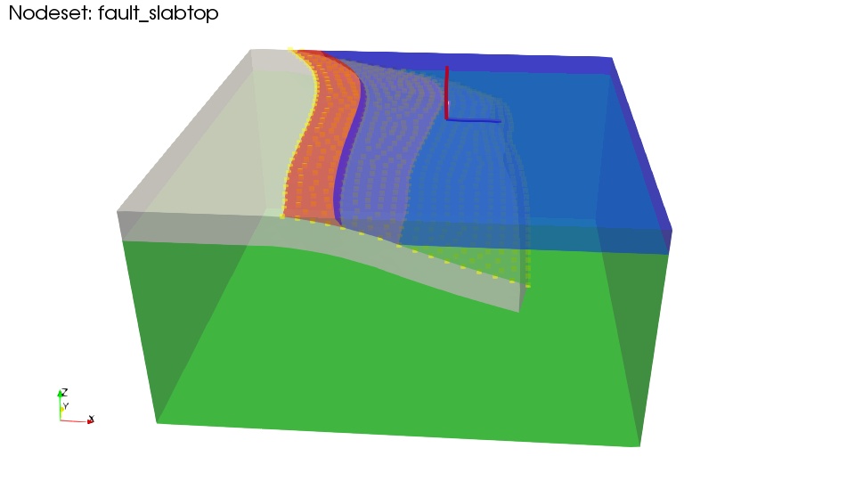
Fig. 99 Visualization of the fault_slabtop nodeset (yellow dots) for the Exodus-II file input/mesh_tet.exo using the viz/plot_mesh.py ParaView Python script. You can step through the different nodesets using the animation controls. This script can also be use to show the mesh quality.