Step 1: Magma inflation#
Features
Quasistatic problem
LU preconditioner
pylith.materials.Poroelasticity
pylith.meshio.MeshIOCubit
pylith.problems.TimeDependent
pylith.problems.SolnDispPresTracStrain
pylith.problems.InitialConditionDomain
pylith.bc.DirichletTimeDependent
pylith.bc.NeumannTimeDependent
pylith.meshio.DataWriterHDF5
spatialdata.spatialdb.SimpleGridDB
spatialdata.spatialdb.UniformDB
Simulation parameter#
This example uses poroelasticity to model flow of magma up through a conduit and into a magma reservoir.
The magma reseroir and conduit have a higher permeability than the surrounding crust.
We generate flow by imposing a pressure on the external boundary of the conduit that is higher than the uniform initial pressure in the domain.
Fig. 110 shows the boundary conditions on the domain.
The parameters specific to this example are in step01_inflation.cfg.

Fig. 110 Boundary and initial conditions for magma inflation. We apply roller boundary conditions on the +x, -x, and -y boundaries. We impose zero pressure (undrained conditions) on the +y boundary and a pressure on the external boundary of the conduit to generate fluid flow.#
[pylithapp.timedependent]
start_time = -0.2*year
initial_dt = 0.2*year
end_time = 10.0*year
[pylithapp.problem]
ic = [domain]
ic.domain = pylith.problems.InitialConditionDomain

[pylithapp.problem.ic.domain]
db = spatialdata.spatialdb.UniformDB
db.description = Initial conditions for domain
db.values = [displacement_x, displacement_y, pressure, trace_strain]
db.data = [0.0*m, 0.0*m, 5.0*MPa, 0.0]
We create an array of 5 Dirichlet boundary conditions: 3 for displacement and 2 for fluid pressure. We have zero displacement perpendicular to the -x, +x, and -y boundaries, zero pressure on the +y boundary, and 10 MPa of fluid pressure on the external boundary of the conduit.
[pylithapp.problem]
bc = [bc_xneg, bc_xpos, bc_yneg, bc_ypos, bc_flow]

bc.bc_xneg = pylith.bc.DirichletTimeDependent
bc.bc_xpos = pylith.bc.DirichletTimeDependent
bc.bc_yneg = pylith.bc.DirichletTimeDependent
bc.bc_ypos = pylith.bc.DirichletTimeDependent
bc.bc_flow = pylith.bc.DirichletTimeDependent

[pylithapp.problem.bc.bc_xneg]
constrained_dof = [0]
label = boundary_xneg
field = displacement
db_auxiliary_field = pylith.bc.ZeroDB
db_auxiliary_field.description = Dirichlet BC -x

[pylithapp.problem.bc.bc_xpos]
constrained_dof = [0]
label = boundary_xpos
field = displacement
db_auxiliary_field = pylith.bc.ZeroDB
db_auxiliary_field.description = Dirichlet BC +x

[pylithapp.problem.bc.bc_yneg]
constrained_dof = [1]
label = boundary_yneg
field = displacement
db_auxiliary_field = pylith.bc.ZeroDB
db_auxiliary_field.description = Dirichlet BC -y

[pylithapp.problem.bc.bc_ypos]
constrained_dof = [0]
label = boundary_ypos
field = pressure
db_auxiliary_field = pylith.bc.ZeroDB
db_auxiliary_field.description = Dirichlet BC +z

[pylithapp.problem.bc.bc_flow]
constrained_dof = [0]
label = boundary_flow
field = pressure
db_auxiliary_field = spatialdata.spatialdb.UniformDB
db_auxiliary_field.description = Flow into external boundary of conduit
db_auxiliary_field.values = [initial_amplitude]
db_auxiliary_field.data = [10.0*MPa]
Running the simulation#
$ pylith step01_inflation.cfg

# The output should look something like the following.
 >> /Users/baagaard/software/unix/py39-venv/pylith-debug/lib/python3.9/site-packages/pylith/meshio/MeshIOObj.py:44:read
 -- meshiocubit(info)
 -- Reading finite-element mesh
 >> /Users/baagaard/src/cig/pylith/libsrc/pylith/meshio/MeshIOCubit.cc:157:void pylith::meshio::MeshIOCubit::_readVertices(pylith::meshio::ExodusII &, pylith::scalar_array *, int *, int *) const
 -- meshiocubit(info)
 -- Component 'reader': Reading 747 vertices.
 >> /Users/baagaard/src/cig/pylith/libsrc/pylith/meshio/MeshIOCubit.cc:217:void pylith::meshio::MeshIOCubit::_readCells(pylith::meshio::ExodusII &, pylith::int_array *, pylith::int_array *, int *, int *) const
 -- meshiocubit(info)
 -- Component 'reader': Reading 705 cells in 2 blocks.
 >> /Users/baagaard/src/cig/pylith/libsrc/pylith/meshio/MeshIOCubit.cc:279:void pylith::meshio::MeshIOCubit::_readGroups(pylith::meshio::ExodusII &)
 -- meshiocubit(info)
 -- Component 'reader': Found 5 node sets.
 >> /Users/baagaard/src/cig/pylith/libsrc/pylith/meshio/MeshIOCubit.cc:305:void pylith::meshio::MeshIOCubit::_readGroups(pylith::meshio::ExodusII &)
 -- meshiocubit(info)
 -- Component 'reader': Reading node set 'boundary_xneg' with id 20 containing 21 nodes.
 >> /Users/baagaard/src/cig/pylith/libsrc/pylith/meshio/MeshIOCubit.cc:305:void pylith::meshio::MeshIOCubit::_readGroups(pylith::meshio::ExodusII &)
 -- meshiocubit(info)
 -- Component 'reader': Reading node set 'boundary_xpos' with id 21 containing 21 nodes.
 >> /Users/baagaard/src/cig/pylith/libsrc/pylith/meshio/MeshIOCubit.cc:305:void pylith::meshio::MeshIOCubit::_readGroups(pylith::meshio::ExodusII &)
 -- meshiocubit(info)
 -- Component 'reader': Reading node set 'boundary_yneg' with id 22 containing 23 nodes.
 >> /Users/baagaard/src/cig/pylith/libsrc/pylith/meshio/MeshIOCubit.cc:305:void pylith::meshio::MeshIOCubit::_readGroups(pylith::meshio::ExodusII &)
 -- meshiocubit(info)
 -- Component 'reader': Reading node set 'boundary_ypos' with id 23 containing 21 nodes.
 >> /Users/baagaard/src/cig/pylith/libsrc/pylith/meshio/MeshIOCubit.cc:305:void pylith::meshio::MeshIOCubit::_readGroups(pylith::meshio::ExodusII &)
 -- meshiocubit(info)
 -- Component 'reader': Reading node set 'boundary_flow' with id 24 containing 3 nodes.
 >> /Users/baagaard/src/cig/pylith/libsrc/pylith/meshio/MeshIO.cc:94:void pylith::meshio::MeshIO::read(topology::Mesh *)
 -- meshiocubit(info)
 -- Component 'reader': Domain bounding box:
    (0, 20000)
    (-20000, 0)
 >> /Users/baagaard/software/unix/py39-venv/pylith-debug/lib/python3.9/site-packages/pylith/problems/Problem.py:116:preinitialize
 -- timedependent(info)
 -- Performing minimal initialization before verifying configuration.
 >> /Users/baagaard/software/unix/py39-venv/pylith-debug/lib/python3.9/site-packages/pylith/problems/Solution.py:44:preinitialize
 -- solution(info)
 -- Performing minimal initialization of solution.
 >> /Users/baagaard/software/unix/py39-venv/pylith-debug/lib/python3.9/site-packages/pylith/problems/Problem.py:175:verifyConfiguration
 -- timedependent(info)
 -- Verifying compatibility of problem configuration.
 >> /Users/baagaard/software/unix/py39-venv/pylith-debug/lib/python3.9/site-packages/pylith/problems/Problem.py:221:_printInfo
 -- timedependent(info)
 -- Scales for nondimensionalization:
    Length scale: 100*m
    Time scale: 6.31152e+06*s
    Pressure scale: 1e+10*m**-1*kg*s**-2
    Density scale: 3.98353e+19*m**-3*kg
    Temperature scale: 1*K
 >> /Users/baagaard/software/unix/py39-venv/pylith-debug/lib/python3.9/site-packages/pylith/problems/Problem.py:186:initialize
 -- timedependent(info)
 -- Initializing timedependent problem with quasistatic formulation.
 >> /Users/baagaard/src/cig/pylith/libsrc/pylith/utils/PetscOptions.cc:235:static void pylith::utils::_PetscOptions::write(pythia::journal::info_t &, const char *, const pylith::utils::PetscOptions &)
 -- petscoptions(info)
 -- Setting PETSc options:
ksp_atol = 1.0e-12
ksp_converged_reason = true
ksp_error_if_not_converged = true
ksp_rtol = 1.0e-12
pc_type = lu
snes_atol = 1.0e-9
snes_converged_reason = true
snes_error_if_not_converged = true
snes_monitor = true
snes_rtol = 1.0e-12
ts_error_if_step_fails = true
ts_monitor = true
ts_type = beuler

# -- many lines ommitted --

50 TS dt 1. time 49.
    0 SNES Function norm 3.049429649018e-03
    Linear solve converged due to CONVERGED_ATOL iterations 1
    1 SNES Function norm 5.567219918314e-16
  Nonlinear solve converged due to CONVERGED_FNORM_ABS iterations 1
51 TS dt 1. time 50.
 >> /Users/baagaard/software/unix/py39-venv/pylith-debug/lib/python3.9/site-packages/pylith/problems/Problem.py:201:finalize
 -- timedependent(info)
 -- Finalizing problem.
At the beginning of the output written to the terminal, we see that PyLith is reading the mesh using the MeshIOCubit reader and that it found the domain to extend from 0 to 20 km in the x direction and from -20 km to 0 in the y direction.
The scales for nondimensionalization .
PyLith detects the use of poroelasticity without a fault and selects appropriate preconditioning options as discussed in PETSc Options.
At the end of the output written to the terminal, we see that the solver advanced the solution 51 time steps.
At each time step, the linear converges in 1 iteration and the norm of the residual met the absolute convergence tolerance (ksp_atol) .
The nonlinear solve converged in 1 iteration, which we expect because this is a linear problem, and the residual met the absolute convergence tolerance (snes_atol).
Visualizing the results#
The output directory contains the simulation output.
Each “observer” writes its own set of files, so the solution over the domain is in one set of files, the boundary condition information is in another set of files, and the material information is in yet another set of files.
The HDF5 (.h5) files contain the mesh geometry and topology information along with the solution fields.
The Xdmf (.xmf) files contain metadata that allow visualization tools like ParaView to know where to find the information in the HDF5 files.
To visualize the data using ParaView or Visit, load the Xdmf files.
In Fig. 111 we use ParaView to visualize the y displacement field using the viz/plot_dispwarp.py Python script.
First, we start ParaView from the examples/magma-2d directory.
$ PATH_TO_PARAVIEW/paraview

# For macOS, it will be something like
$ /Applications/ParaView-5.10.1.app/Contents/MacOS/paraview
Next we run the viz/plot_dispwarp.py Python script as described in ParaView Python Scripts.
For Step 1 we do not need to change any of the default values.
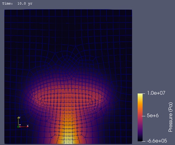
Fig. 111 Solution for Step 1 at t=100 yr. The colors of the shaded surface indicate the fluid pressure, and the deformation is exaggerated by a factor of 1000.#