Step 5: Time-Dependent Shear Displacement and Tractions#
In this example we build on Step 3 and make the Dirichlet (displacement) and Neumann (traction) boundary conditions a bit more complicated by adding variation in time. The simulation has a duration of 5 years with a time step of 1 year. The time-dependent boundary conditions use the same initial amplitude values for the first time step before adding in a constant rate increase at a time of 1 year. Fig. 46 shows the boundary conditions on the domain.

Fig. 46 Boundary conditions for shear deformation. We constrain the x and y displacements on the +x and -x boundaries. We apply tangential (shear) tractions on the +y and -y boundaries. At a time of 1 year we increase the amplitude at a constrant rate \(b\) (\(H(t)\) corresponds to the heavyside step function).#
Features
Tetrahedral cells
pylith.meshio.MeshIOPetsc
pylith.problems.TimeDependent
pylith.materials.Elasticity
pylith.materials.IsotropicLinearElasticity
spatialdata.spatialdb.UniformDB
pylith.meshio.OutputSolnBoundary
pylith.meshio.DataWriterHDF5
Quasistatic simulation
backward Euler time stepping
ILU preconditioner
pylith.bc.DirichletTimeDependent
pylith.bc.NeumannTimeDependent
spatialdata.spatialdb.SimpleDB
spatialdata.spatialdb.ZeroDB
Simulation parameters#
The parameters specific to this example are in step05_sheardisptractrate.cfg.
This is a time-dependent problem, so we must specify the start and end times of the simulation along with the initial time step.
With an initial time step of 1 year, we start the simulation at -1 year so that the first solve will advance the simulation to a time of 0.
We also specify a relaxation time on the order of the time scale of the simulation to allow for reasonable nondimensionalization of time.
$ pylith step05_sheardisptractrate.cfg

# The output should look something like the following.
 >> /software/unix/py39-venv/pylith-debug/lib/python3.9/site-packages/pylith/meshio/MeshIOObj.py:44:read
 -- meshiopetsc(info)
 -- Reading finite-element mesh
 >> /src/cig/pylith/libsrc/pylith/meshio/MeshIO.cc:94:void pylith::meshio::MeshIO::read(topology::Mesh *)
 -- meshiopetsc(info)
 -- Component 'reader': Domain bounding box:
    (-6000, 6000)
    (-6000, 6000)
    (-9000, 0)

# -- many lines omitted --

5 TS dt 0.1 time 0.4
    0 SNES Function norm 7.135615733940e-03
    Linear solve converged due to CONVERGED_ATOL iterations 1
    1 SNES Function norm 1.130764208982e-17
  Nonlinear solve converged due to CONVERGED_FNORM_ABS iterations 1
6 TS dt 0.1 time 0.5
 >> /software/baagaard/py38-venv/pylith-debug/lib/python3.8/site-packages/pylith/problems/Problem.py:201:finalize
 -- timedependent(info)
 -- Finalizing problem.
The output written to the terminal now contains multiple time steps. The PETSc TS (time stepping) monitor shows the time step and time in nondimensional units.
Visualizing the results#
In Fig. 44 we use ParaView to visualize the x displacement field using the viz/plot_dispwarp.py Python script.
As in Step 2 we override the default name of the simulation file with the name of the current simulation before running the viz/plot_dispwarp.py Python script.
>>> SIM = "step05_sheardisptractrate"
One you run the viz/plot_dispwarp.py Python script, you can click on the “play” button corresponding to the right triangle in the toolbar to view the time-dependent deformation.
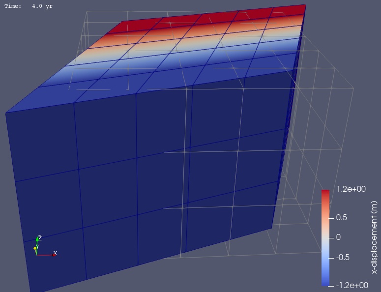
Fig. 47 Solution for Step 5 at a time of 4.0 years. The colors of the shaded surface indicate the magnitude of the x displacement, and the deformation is exaggerated by a factor of 1000. The undeformed configuration is show by the gray wireframe.#