Step 3: Shear Displacement and Tractions

In Step 3 we replace the Dirichlet (displacement) boundary conditions on the +y and -y boundaries with equivalent Neumann (traction) boundary conditions. In order to maintain symmetry and prevent rigid body motion, we constrain both the x and y displacements on the +x and -x boundaries. The solution matches that in Step 2. Fig. 43 shows the boundary conditions on the domain.

Fig. 43 Boundary conditions for shear deformation. We constrain the x and y displacements on the +x and -x boundaries. We apply tangential (shear) tractions on the +y and -y boundaries.

Features

• Tetrahedral cells

• pylith.meshio.MeshIOPetsc

• pylith.problems.TimeDependent

• pylith.materials.Elasticity

• pylith.materials.IsotropicLinearElasticity

• spatialdata.spatialdb.UniformDB

• pylith.meshio.OutputSolnBoundary

• pylith.meshio.DataWriterHDF5

• Static simulation

• ILU preconditioner

• pylith.bc.DirichletTimeDependent

• pylith.bc.NeumannTimeDependent

• spatialdata.spatialdb.SimpleDB

• spatialdata.spatialdb.ZeroDB

Simulation parameters

The parameters specific to this example are in step03_sheardisptract.cfg.

The primary change from Step 2 is the use of Neumann (traction) boundary conditions in pylith.problem.bc. The tractions are uniform on each of the two boundaries, so we use a UniformDB. In PyLith the direction of the tangential tractions in 2D is defined by the cross product of the +z direction and the outward normal on the boundary. On the +y boundary a positive tangential traction is in the -x direction, and on the -y boundary a positive tangential traction is in the +x direction. We want tractions in the opposite direction as shown by the arrows in Fig. 43, so we apply negative tangential tractions.

Listing 39 Run Step 3 simulation

$ pylith step03_sheardisptract.cfg

# The output should look something like the following.
 >> /software/unix/py39-venv/pylith-debug/lib/python3.9/site-packages/pylith/meshio/MeshIOObj.py:44:read
 -- meshiopetsc(info)
 -- Reading finite-element mesh
 >> /src/cig/pylith/libsrc/pylith/meshio/MeshIO.cc:94:void pylith::meshio::MeshIO::read(topology::Mesh *)
 -- meshiopetsc(info)
 -- Component 'reader': Domain bounding box:
    (-6000, 6000)
    (-6000, 6000)
    (-9000, 0)

# -- many lines omitted --

 >> /software/baagaard/py38-venv/pylith-debug/lib/python3.8/site-packages/pylith/problems/TimeDependent.py:139:run
 -- timedependent(info)
 -- Solving problem.
0 TS dt 0.01 time 0.
    0 SNES Function norm 2.854246293576e-02 
    Linear solve converged due to CONVERGED_ATOL iterations 1
    1 SNES Function norm 2.511862662012e-17 
  Nonlinear solve converged due to CONVERGED_FNORM_ABS iterations 1
1 TS dt 0.01 time 0.01
 >> /software/baagaard/py38-venv/pylith-debug/lib/python3.8/site-packages/pylith/problems/Problem.py:201:finalize
 -- timedependent(info)
 -- Finalizing problem.

The output written to the terminal is nearly identical to what we saw for Step 2. The linear solve did require only 7 iteration to converge.

Visualizing the results

In Fig. 44 we use ParaView to visualize the x displacement field using the viz/plot_dispwarp.py Python script. As in Step 2 we override the default name of the simulation file with the name of the current simulation before running the viz/plot_dispwarp.py Python script.

Listing 40 Set the simulation in the ParaView Python Shell.

>>> SIM = "step03_sheardisptract"

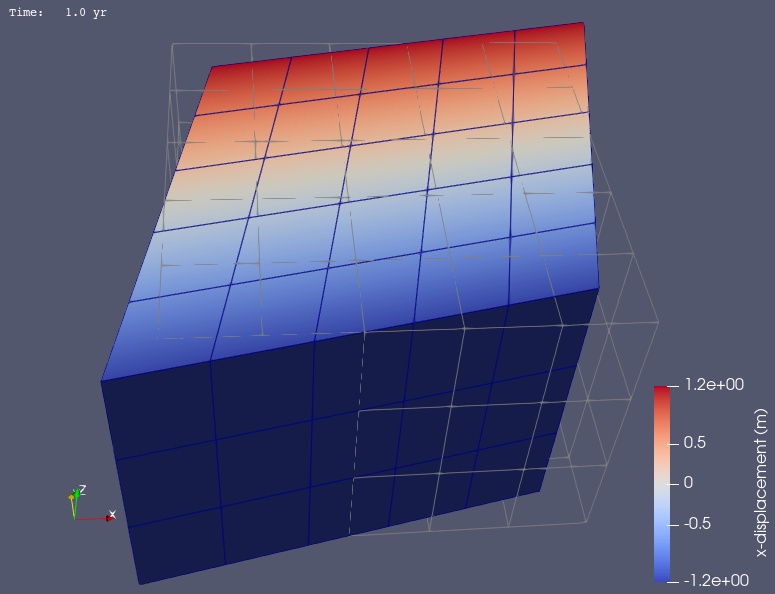
Fig. 44 Solution for Step 3. The colors of the shaded surface indicate the magnitude of the x displacement, and the deformation is exaggerated by a factor of 1000. The undeformed configuration is show by the gray wireframe. The solution matches the one from Step 2.