
Step 2: No faults with flexure#
Features
Quasi-static problem
triangular cells
LU preconditioner
pylith.materials.Poroelasticity
pylith.meshio.MeshIOPetsc
pylith.problems.TimeDependent
pylith.problems.SolnDispPresTracStrainVelPdotTdot
pylith.problems.InitialConditionDomain
pylith.bc.DirichletTimeDependent
pylith.bc.NeumannTimeDependent
pylith.meshio.DataWriterHDF5
spatialdata.spatialdb.SimpleGridDB
Simulation parameters#
This example uses poroelasticity to model the infiltration of seawater through a slab of oceanic lithosphere. The permeability field is depth dependent, decreasing with depth but does not vary laterally. The lithosphere is now subject to deformation, over 300 kyr the slab bends to simulate extensional stresses in the outer-rise of a subduction zone. A fluid pressure is applied to the top boundary that is equivalent to the pressure exerted on the seafloor by the water column. This simulates what the hydration state of the oceanic lithosphere as it is about to enter a convergent margin.
Fig. 177 shows the boundary conditions on the domain.
The parameters specific to this example are in step02_no_faults_flexure.cfg.

Fig. 177 Boundary and initial conditions for Step 2.
We fix the left boundary, but we now apply a spatially varying velocity condition on the top boundary using a SimpleDB file, while leaving the right and bottom boundaries unconstrained.
We impose a fluid pressure on the +y boundary equal to the weight of the water column to generate fluid flow.#
[pylithapp.problem.bc.boundary_top]
use_initial = False
use_rate = True

db_auxiliary_field = spatialdata.spatialdb.SimpleDB
db_auxiliary_field.description = Dirichlet BC +y boundary
db_auxiliary_field.iohandler.filename = top_velocity_boundary.spatialdb
SimpleGridDB file that does not contain enhanced permeability due to outer rise faults.#[pylithapp.problem]
[pylithapp.problem.materials.slab]
db_auxiliary_field.filename = no_faultzone_permeability.spatialdb
Running the simulation#
$ pylith step02_no_faults_flexure.cfg
>> software/pylith-debug/lib/python3.12/site-packages/pylith/apps/PyLithApp.py:79:main
-- info (application-flow)
-- Running on 1 process(es).

# -- many lines omitted --
>> src/cig/pylith/libsrc/pylith/problems/TimeDependent.cc:473:void pylith::problems::TimeDependent::solve()
-- info (application-flow)
-- Component 'timedependent.problem': Solving equations.
0 TS dt 8.41536 time -8.41536
    0 SNES Function norm 1.780933174156e+03
      Linear solve converged due to CONVERGED_ATOL iterations 23
    1 SNES Function norm 9.489171115501e-10
    Nonlinear solve converged due to CONVERGED_FNORM_ABS iterations 1
1 TS dt 8.41536 time 0.
    0 SNES Function norm 1.624022924774e+03
      Linear solve converged due to CONVERGED_ATOL iterations 34
    1 SNES Function norm 1.245577106021e-08
    Nonlinear solve converged due to CONVERGED_FNORM_ABS iterations 1

# -- many lines omitted --

50 TS dt 8.41536 time 412.353
    0 SNES Function norm 1.624022924815e+03
      Linear solve converged due to CONVERGED_ATOL iterations 36
    1 SNES Function norm 8.879603719365e-09
    Nonlinear solve converged due to CONVERGED_FNORM_ABS iterations 1
51 TS dt 8.41536 time 420.768
>> software/pylith-debug/lib/python3.12/site-packages/pylith/problems/Problem.py:222:finalize
-- info (application-flow)
-- Finalizing problem.
Visualizing the results#
In Fig. 178 we use the pylith_viz utility to visualize the porosity field.
pylith_viz --filenames=output/step02_no_faults_flexure-slab.h5 warp_grid --field=porosity --exaggeration=1 --hide-edges
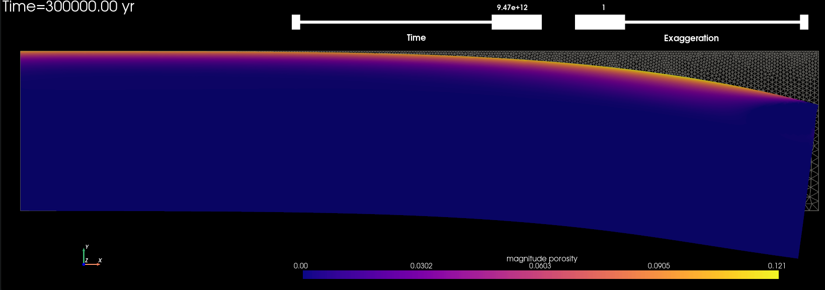
Fig. 178 Porosity field at the end of the simulation for Step 2.#