
Step 2: Static Spatially Variable Coseismic Slip#
Features
Triangular cells
pylith.problems.TimeDependent
pylith.materials.Elasticity
pylith.materials.IsotropicLinearElasticity
pylith.faults.FaultCohesiveKin
pylith.faults.KinSrcStep
pylith.bc.DirichletTimeDependent
spatialdata.spatialdb.UniformDB
pylith.meshio.OutputSolnBoundary
pylith.meshio.DataWriterHDF5
Static simulation
pylith.meshio.MeshIOPetsc
Gmsh
spatially variable slip
Simulation parameters#
This example involves a static simulation that solves for the deformation from prescribed spatially variable coseismic slip on each of the faults.
Fig. 120 shows the boundary conditions on the domain.
The parameters specific to this example are in step02_varslip.cfg.

Fig. 120 Boundary conditions for static coseismic slip. On the boundary of the domain, we set the displacement component that is perpendicular to the boundary to zero. We prescribe piecewise linear variations in slip along strike on each of the faults.#
We prescribe piecewise linear variations in slip along strike on each of the faults using SimpleDB spatial databases.
The spatial databases contain coordinates of points in geographic coordinates.
PyLith will transform each the coordinates of point on the fault to the geographic coordinates and interpolate the values in the spatial database to the point on the fault.
[pylithapp.problem.interfaces.main_fault.eq_ruptures.rupture]
db_auxiliary_field = spatialdata.spatialdb.SimpleDB
db_auxiliary_field.description = Slip parameters for fault 'main'
db_auxiliary_field.iohandler.filename = fault_main_slip.spatialdb
db_auxiliary_field.query_type = linear

[pylithapp.problem.interfaces.west_branch.eq_ruptures.rupture]
db_auxiliary_field = spatialdata.spatialdb.SimpleDB
db_auxiliary_field.description = Slip parameters for fault 'west'
db_auxiliary_field.iohandler.filename = fault_west_slip.spatialdb
db_auxiliary_field.query_type = linear

[pylithapp.problem.interfaces.east_branch.eq_ruptures.rupture]
db_auxiliary_field = spatialdata.spatialdb.SimpleDB
db_auxiliary_field.description = Slip parameters for fault 'east'
db_auxiliary_field.iohandler.filename = fault_east_slip.spatialdb
db_auxiliary_field.query_type = linear
Running the simulation#
$ pylith step02_varslip.cfg

# The output should look something like the following.
>> software/pylith-debug/lib/python3.12/site-packages/pylith/apps/PyLithApp.py:79:main
-- info (application-flow)
-- Running on 1 process(es).

# -- many lines removed --
>> src/cig/pylith/libsrc/pylith/problems/TimeDependent.cc:473:void pylith::problems::TimeDependent::solve()
-- info (application-flow)
-- Component 'timedependent.problem': Solving equations.
0 TS dt 0.001 time 0.
    0 SNES Function norm 1.139546193525e+01
      Linear solve converged due to CONVERGED_ATOL iterations 13
    1 SNES Function norm 3.278661158667e-08
    Nonlinear solve converged due to CONVERGED_FNORM_ABS iterations 1
1 TS dt 0.001 time 0.001
>> software/pylith-debug/lib/python3.12/site-packages/pylith/problems/Problem.py:222:finalize
-- info (application-flow)
-- Finalizing problem.
At the end of the output written to the terminal, we see that the solver advanced the solution one time step (static simulation).
The linear solve converged after 13 iterations and the norm of the residual met the absolute convergence tolerance (ksp_atol) .
The nonlinear solve converged in 1 iteration, which we expect because this is a linear problem, and the residual met the absolute convergence tolerance (snes_atol).
Visualizing the results#
In Fig. 121 we use the pylith_viz utility to visualize the y displacement field.
pylith_viz --filename=output/step02_varslip-domain.h5 warp_grid --component=y
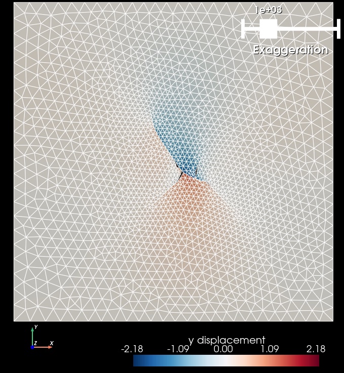
Fig. 121 Solution for Step 2. The colors of the shaded surface indicate the y displacement, and the deformation is exaggerated by a factor of 1000. The undeformed configuration is shown by the gray wireframe. The contrast in material properties across the faults causes the asymmetry in the y displacement field.#