Step 3: Shear Displacement and Tractions

Features

• Quadrilateral cells

• pylith.meshio.MeshIOAscii

• pylith.problems.TimeDependent

• pylith.materials.Elasticity

• pylith.materials.IsotropicLinearElasticity

• spatialdata.spatialdb.UniformDB

• pylith.meshio.DataWriterHDF5

• Static simulation

• LU preconditioner

• pylith.bc.DirichletTimeDependent

• pylith.bc.NeumannTimeDependent

• spatialdata.spatialdb.SimpleDB

Simulation parameters

In Step 3 we replace the Dirichlet (displacement) boundary conditions on the +y and -y boundaries with equivalent Neumann (traction) boundary conditions. In order to maintain symmetry and prevent rigid body motion, we constrain both the x and y displacements on the +x and -x boundaries. The solution matches that in Step 2. Fig. 31 shows the boundary conditions on the domain. The parameters specific to this example are in step03_sheardisptract.cfg.

Fig. 31 Boundary conditions for shear deformation. We constrain the x and y displacements on the +x and -x boundaries. We apply tangential (shear) tractions on the +y and -y boundaries.

The tractions are uniform on each of the two boundaries, so we use a UniformDB. In PyLith the direction of the tangential tractions in 2D is defined by the cross product of the +z direction and the outward normal on the boundary. On the +y boundary a positive tangential traction is in the -x direction, and on the -y boundary a positive tangential traction is in the +x direction. We want tractions in the opposite direction as shown by the arrows in Fig. 31, so we apply negative tangential tractions.

Listing 41 Specifying the boundary conditions for Step 3. We only show the detailed settings for the -x and -y boundaries.

[pylithapp.problem]
bc = [bc_xneg, bc_yneg, bc_xpos, bc_ypos]
bc.bc_xneg = pylith.bc.DirichletTimeDependent
bc.bc_xpos = pylith.bc.DirichletTimeDependent
bc.bc_yneg = pylith.bc.NeumannTimeDependent
bc.bc_ypos = pylith.bc.NeumannTimeDependent

[pylithapp.problem.bc.bc_xneg]
# Degrees of freedom (dof) 0 and 1 correspond to the x and y displacements. 
constrained_dof = [0, 1]
label = boundary_xneg
db_auxiliary_field = spatialdata.spatialdb.SimpleDB
db_auxiliary_field.description = Dirichlet BC -x boundary
db_auxiliary_field.iohandler.filename = sheardisp_bc_xneg.spatialdb
db_auxiliary_field.query_type = linear

[pylithapp.problem.bc.bc_yneg]
label = boundary_yneg
db_auxiliary_field = spatialdata.spatialdb.UniformDB
db_auxiliary_field.description = Neumann BC -y boundary
db_auxiliary_field.values = [initial_amplitude_tangential, initial_amplitude_normal]
db_auxiliary_field.data = [-4.5*MPa, 0*MPa]

Running the simulation

Listing 42 Run Step 3 simulation

$ pylith step03_sheardisptract.cfg

# The output should look something like the following.
 >> software/pylith-debug/lib/python3.12/site-packages/pylith/apps/PyLithApp.py:79:main
 -- info (application-flow)
 -- Running on 1 process(es).

# -- many lines omitted --

 >> src/cig/pylith/libsrc/pylith/problems/TimeDependent.cc:473:void pylith::problems::TimeDependent::solve()
 -- info (application-flow)
 -- Component 'timedependent.problem': Solving equations.
0 TS dt 0.001 time 0.
    0 SNES Function norm 1.817939142477e+01
      Linear solve converged due to CONVERGED_ATOL iterations 3
    1 SNES Function norm 8.280473801872e-08
    Nonlinear solve converged due to CONVERGED_FNORM_ABS iterations 1
1 TS dt 0.001 time 0.001
 >> software/pylith-debug/lib/python3.12/site-packages/pylith/problems/Problem.py:222:finalize
 -- info (application-flow)
 -- Finalizing problem.

As expected, the output written to the terminal is nearly identical to what we saw for Steps 1 and 2.

Visualizing the results

In Fig. 32 we use the pylith_viz utility to visualize the x displacement field.

Listing 43 Visualize PyLith output using pylith_viz.

pylith_viz --filenames=output/step03_sheardisptract-domain.h5 warp_grid --component=x

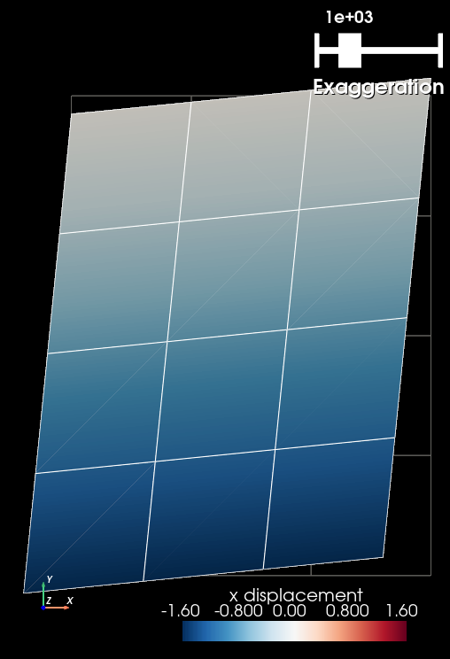
Fig. 32 Solution for Step 3. The colors of the shaded surface indicate the x displacement, and the deformation is exaggerated by a factor of 1000. The undeformed configuration is shown by the gray wireframe. The solution matches the one from Step 2.