Strike-Slip Benchmark#

This benchmark problem computes the viscoelastic (Maxwell) relaxation of stresses from a single, finite, strike-slip earthquake in 3D without gravity. Dirichlet boundary conditions equal to the analytical elastic solution are imposed on the sides of a cube with sides of length 24 km. Anti-plane strain boundary conditions are imposed at y = 0, so the solution is equivalent to that for a domain with a 48 km length in the y direction. We can use the analytical solution of Okada [1992] both to apply the boundary conditions and to compare against the numerically-computed elastic solution.

Problem Description#

Fig. 119 shows the geometry of the strike-slip fault (red surface) embedded in the cube consisting of an elastic material (yellow block) over a Maxwell viscoelastic material (blue block).

Domain The domain spans the region

(179)#\[\begin{gather} 0\leq x\leq24\ km,\\ 0\leq y\leq24\ km,\\ -24\ km\leq z\leq0. \end{gather}\]

The top (elastic) layer occupies the region \(-12\ km\ \leq z\leq0\) and the bottom (viscoelastic) layer occupies the region \(-24\ km\ \leq z\leq-12\ km\).

Material properties The material is a Poisson solid with a shear modulus of 30 GPa. The domain is modeled using an elastic isotropic material for the top layer and a Maxwell viscoelastic material for the bottom layer. The bottom layer has a viscosity of 1.0e+18 Pa-s.

Fault The fault is a vertical, right-lateral strike-slip fault. The strike is parallel to the y-direction at the center of the model:

(180)#\[\begin{gather} x=12\ km,\\ 0\leq y\leq16\ km,\\ -16\ km\leq z\leq0. \end{gather}\]

Uniform slip of 1 m is applied over the region \(0\leq y\leq12\ km\) and \(-12\ km\leq z\leq0\) with a linear taper to 0 at y = 16 km and z = -16 km. The tapered region is the light red portion of the fault surface in Fig. 119. In the region where the two tapers overlap, each slip value is the minimum of the two tapers (so that the taper remains linear).

Boundary conditions Bottom and side displacements are set to the elastic analytical solution, and the top of the model is a free surface. There are two exceptions to these applied boundary conditions. The first is on the y=0 plane, where y-displacements are left free to preserve symmetry, and the x- and z-displacements are set to zero. The second is along the line segment between (12, 0, -24) and (12, 24, -24), where the analytical solution blows up in some cases. Along this line segment, all three displacement components are left free.

Discretization The model is discretized with nominal spatial resolutions of 1000 m, 500 m, and 250 m.

Basis functions We use trilinear hexahedral cells and linear tetrahedral cells.

Solution We compute the error in the elastic solution and compare the solution over the domain after 0, 1, 5, and 10 years.

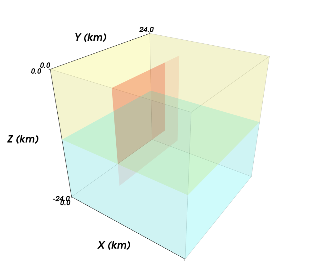
Fig. 119 Geometry of strike-slip benchmark problem.#

Running the Benchmark#

Each benchmark uses three .cfg files in the parameters directory: pylithapp.cfg, a mesher related file ( strikeslip_cubit.cfg), and a resolution and cell related file (e.g., strikeslip_hex8_1000m.cfg).

# Checkout the benchmark files from the CIG Git repository.
$ git clone https://github.com/geodynamics/pylith_benchmarks.git
# Change to the quasistatic/sceccrustdeform/strikeslip directory.
$ cd quasistatic/sceccrustdeform/strikeslip
# Decompress the gzipped files in the meshes and parameters directories.
$ gunzip meshes/*.gz parameters/*.gz
# Change to the parameters directory.
$ cd parameters
# Examples of running static (elastic solution only) cases.
$ pylith strikeslip_cubit.cfg strikeslip_hex8_1000m.cfg
$ pylith strikeslip_cubit.cfg strikeslip_hex8_0500m.cfg
$ pylith strikeslip_cubit.cfg strikeslip_tet4_1000m.cfg
# Append timedep.cfg to run the time-dependent (viscoelastic cases).
$ pylith strikeslip_cubit.cfg strikeslip_hex8_1000m.cfg timedep.cfg
$ pylith strikeslip_cubit.cfg strikeslip_hex8_0500m.cfg timedep.cfg
$ pylith strikeslip_cubit.cfg strikeslip_tet4_1000m.cfg timedep.cfg

This will run the problem for 10 years, using a time-step size of 0.1 years, and results will be output for each year. The benchmarks at resolutions of 1000 m, 500 m, and 250 m require approximately 150 MB, 960 MB, and 8 GB, respectively.

Benchmark Results#

Fig. 120 shows the displacement field from the simulation with hexahedral cells using trilinear basis functions at a resolution of 1000 m. For each resolution and set of basis functions, we measure the accuracy by comparing the numerical solution against the semi-analytical Okada solution [Okada, 1992]. We also compare the accuracy and runtime across resolutions and different cell types. This provides practical information about what cell types and resolutions are required to achieve a given level of accuracy with the shortest runtime.

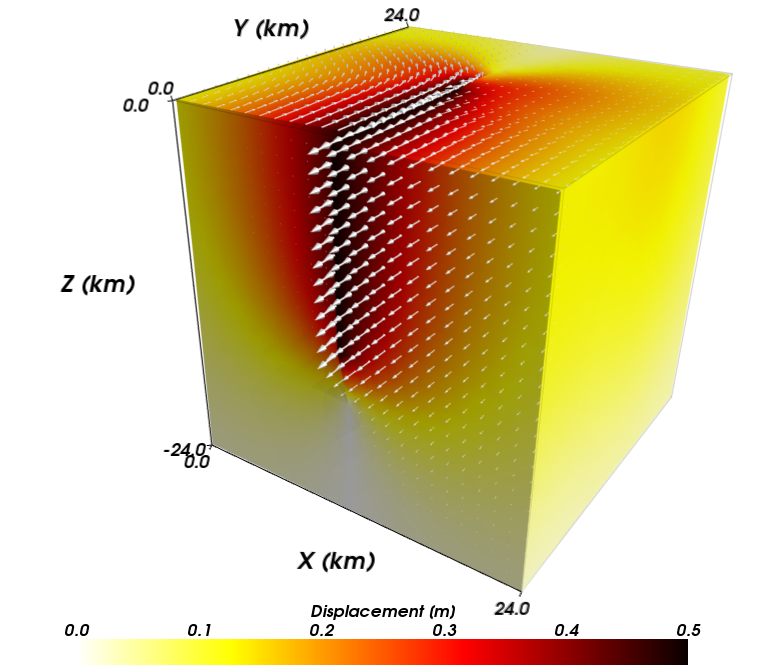
Fig. 120 Displacement field for strike-slip benchmark problem.#

Solution Accuracy#

We quantify the error in the finite-element solution by integrating the L2 norm of the difference between the finite-element solution and the semi-analytical solution evaluated at the quadrature points. We define the local error (error for each finite-element cell) to be

(181)#\[\begin{equation} \epsilon_{local}=\frac{1}{V_{cell}}\sqrt{\intop_{cell}\left(u_{i}^{t}-u_{i}^{fem}\right)^{2}\: dV}, \end{equation}\]

where \(u_{i}^{t}\) is the ith component of the displacement field for the semi-analytical solution, and \(u_{i}^{fem}\) is the ith component of the displacement field for the finite-element solution. Taking the square root of the L2 norm and normalizing by the volume of the cell results in an error metric with dimensions of length. This roughly corresponds to the error in the magnitude of the displacement field in the finite element solution. We define the global error in a similar fashion,

(182)#\[\begin{equation} \epsilon_{global}=\frac{1}{V_{domain}}\sqrt{\intop_{domain}\left(u_{i}^{t}-u_{i}^{fem}\right)^{2}\: dV}, \end{equation}\]

where we sum the L2 norm computed for the local error over all of the cells before taking the square root and dividing by the volume of the domain.

Figures Fig. 121 through Fig. 126 show the local error for each of the three resolutions and two cell types. The error decreases with decreasing cell size as expected for a converging solution. The largest errors, which approach 1 mm for 1 m of slip for a discretization size of 250 m, occur where the gradient in slip is discontinuous at the boundary between the region of uniform slip and linear taper in slip. The linear basis functions cannot match this higher order variation. The trilinear basis functions in the hexahedral element provide more terms in the polynomial defining the variation in the displacement field within each cell compared to the linear basis functions for the tetrahedral cell. Consequently, for this problem the error for the hexahedral cells at a given resolution is smaller than that for the tetrahedral cells. Both sets of cell types and basis functions provide the same rate of convergence as shown in Fig. 127.

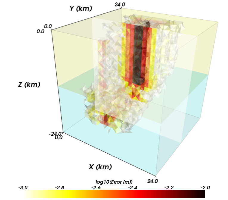
Fig. 121 Local error for strike-slip benchmark problem with tetrahedral cells and linear basis functions with a uniform discretization size of 1000 m.#

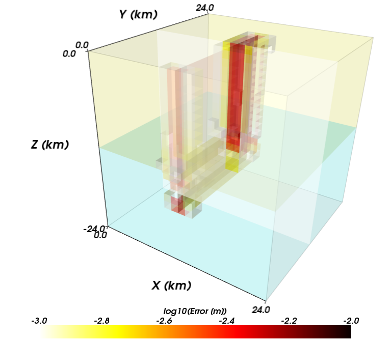
Fig. 122 Local error for strike-slip benchmark problem with hexahedral cells and trilinear basis functions with a uniform discretization size of 1000 m.#

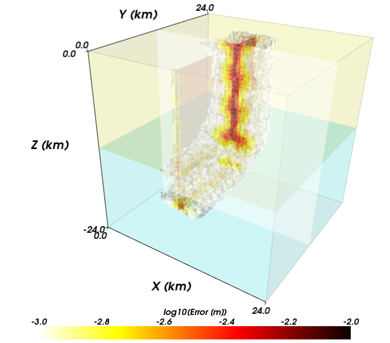
Fig. 123 Local error for strike-slip benchmark problem with tetrahedral cells and linear basis functions with a uniform discretization size of 500 m.#

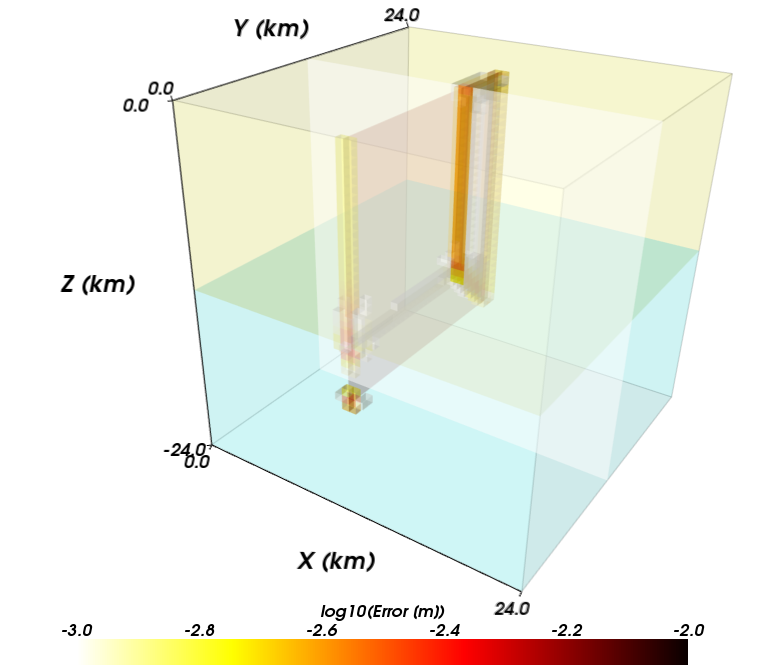
Fig. 124 Local error for strike-slip benchmark problem with hexahedral cells and trilinear basis functions with a uniform discretization size of 500 m.#

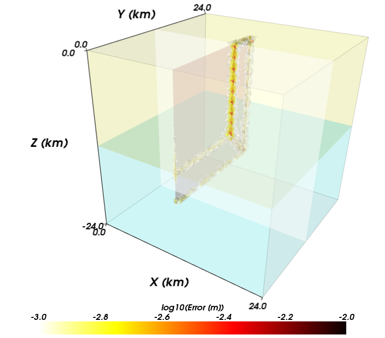
Fig. 125 Local error for strike-slip benchmark problem with tetrahedral cells and linear basis functions with a uniform discretization size of 250 m.#

Fig. 126 Local error for strike-slip benchmark problem with hexahedral cells and trilinear basis functions with a uniform discretization size of 250 m.#

Fig. 127 Convergence rate for the strike-slip benchmark problem with tetrahedral cells and linear basis functions and with hexahedral cells with trilinear basis functions.#

Performance#

Fig. 128 summarizes the overall performance of each of the six simulations. Although at a given resolution, the number of degrees of freedom in the hexahedral and tetrahedral meshes are the same, the number of cells in the tetrahedral mesh is about six times greater. However, we use only one integration point per tetrahedral cell compared to eight for the hexahedral cell. This leads to approximately the same number of integration points for the two meshes, but the time required to unpack/pack information for each cell from the finite-element data structure is greater than the time required to do the calculation for each quadrature point (which can take advantage of the very fast, small memory cache in the processor). As a result, the runtime for the simulations with hexahedral cells is significantly less than that for the tetrahedral cells at the same resolution.

Fig. 129 compares the runtime for the benchmark (elastic solution only) at 500 m resolution for 1 to 16 processors. The total runtime is the time required for the entire simulation, including initialization, distributing the mesh over the processors, solving the problem in parallel, and writing the output to VTK files. Some initialization steps, writing the output to VTK files, and distributing the mesh are essentially serial processes. For simulations with many time steps these steps will generally occupy only a fraction of the runtime, and the runtime will be dominated by the solution of the equations. Fig. 129 also shows the total time required to form the Jacobian of the system, form the residual, and solve the system. These steps provide a more accurate representation of the parallel-performance of the computational portion of the code and show excellent performance as evident in the approximately linear slope of 0.7. A linear decrease with a slope of 1 would indicate strong scaling, which is rarely achieved in real applications.

Fig. 129 Parallel performance of PyLith for the strike-slip benchmark problem with tetrahedral cells and linear basis functions with a uniform discretization size of 500 m. The total runtime (total) and the runtime to compute the Jacobian and residual and solve the system (compute) are shown. The compute runtime decreases with a slope of about 0.7; a linear decrease with a slope of 1 would indicate strong scaling, which is rarely achieved in any real application.#