
Step 2: Static Spatially Variable Coseismic Slip#
Features
Tetrahedral cells
pylith.problems.TimeDependent
pylith.materials.Elasticity
pylith.materials.IsotropicLinearElasticity
pylith.faults.FaultCohesiveKin
pylith.faults.KinSrcStep
pylith.bc.DirichletTimeDependent
spatialdata.spatialdb.UniformDB
pylith.meshio.OutputSolnBoundary
pylith.meshio.DataWriterHDF5
Static simulation
pylith.meshio.MeshIOPetsc
Gmsh
spatially variable slip
Simulation parameters#
This example involves a static simulation that solves for the deformation from prescribed spatially varying coseismic slip on each of the faults.
Fig. 126 shows the boundary conditions on the domain.
The parameters specific to this example are in step02_varslip.cfg.

Fig. 126 Boundary conditions for static coseismic slip. On the boundary of the domain, we set the displacement component that is perpendicular to the boundary to zero. We prescribe slip that varies linearly over each of the fault surfaces.#
We prescribe piecewise linear variations in slip along strike on each of the faults using SimpleDB spatial databases
The spatial databases contain coordinates of points in geographic coordinates.
PyLith will transform each the coordinates of point on the fault to the geographic coordinates and interpolate the values in the spatial database to the point on the fault.
Tip
In most cases you will not want the interpolation to be done in geographic coordinates, because distances in each of the coordinate directions are different. This is especially true when horizontal coordinates are given in longitude and latitude and vertical distances are given in meters. Transforming the points to a geographic projection is generally preferred.
[pylithapp.problem.interfaces.main_fault.eq_ruptures.rupture]
db_auxiliary_field = spatialdata.spatialdb.SimpleDB
db_auxiliary_field.description = Slip parameters for fault 'main'
db_auxiliary_field.iohandler.filename = fault_main_slip.spatialdb
db_auxiliary_field.query_type = linear

[pylithapp.problem.interfaces.west_branch.eq_ruptures.rupture]
db_auxiliary_field = spatialdata.spatialdb.SimpleDB
db_auxiliary_field.description = Slip parameters for fault 'west'
db_auxiliary_field.iohandler.filename = fault_west_slip.spatialdb
db_auxiliary_field.query_type = linear

[pylithapp.problem.interfaces.east_branch.eq_ruptures.rupture]
db_auxiliary_field = spatialdata.spatialdb.SimpleDB
db_auxiliary_field.description = Slip parameters for fault 'east'
db_auxiliary_field.iohandler.filename = fault_east_slip.spatialdb
db_auxiliary_field.query_type = linear
Running the simulation#
$ pylith step02_varslip.cfg

# The output should look something like the following.
 >> /software/unix/py3.12-venv/pylith-debug/lib/python3.12/site-packages/pylith/apps/PyLithApp.py:77:main
 -- pylithapp(info)
 -- Running on 1 process(es).
 >> /software/unix/py3.12-venv/pylith-debug/lib/python3.12/site-packages/pylith/meshio/MeshIOObj.py:38:read
 -- meshiopetsc(info)
 -- Reading finite-element mesh
 >> /src/cig/pylith/libsrc/pylith/meshio/MeshIO.cc:85:void pylith::meshio::MeshIO::read(pylith::topology::Mesh *, const bool)
 -- meshiopetsc(info)
 -- Component 'reader': Domain bounding box:
    (413700, 493700)
    (3.917e+06, 3.977e+06)
    (-40000, 0)

-- many lines omitted --

 >> /software/unix/py3.12-venv/pylith-debug/lib/python3.12/site-packages/pylith/problems/Problem.py:185:initialize
 -- timedependent(info)
 -- Initializing timedependent problem with quasistatic formulation.
 >> /src/cig/pylith/libsrc/pylith/utils/PetscOptions.cc:239:static void pylith::utils::_PetscOptions::write(pythia::journal::info_t &, const char *, const PetscOptions &)
 -- petscoptions(info)
 -- Setting PETSc options:
ksp_converged_reason = true
ksp_guess_pod_size = 8
ksp_guess_type = pod
snes_converged_reason = true
snes_monitor = true
ts_error_if_step_fails = true
ts_monitor = true

 >> /src/cig/pylith/libsrc/pylith/utils/PetscOptions.cc:239:static void pylith::utils::_PetscOptions::write(pythia::journal::info_t &, const char *, const PetscOptions &)
 -- petscoptions(info)
 -- Using user values rather then the following default PETSc options:
ksp_atol = 1.0e-12
ksp_error_if_not_converged = true
ksp_rtol = 1.0e-12
snes_atol = 1.0e-9
snes_error_if_not_converged = true
snes_rtol = 1.0e-12

 >> /software/unix/py3.12-venv/pylith-debug/lib/python3.12/site-packages/pylith/problems/TimeDependent.py:132:run
 -- timedependent(info)
 -- Solving problem.
0 TS dt 0.01 time 0.
    0 SNES Function norm 1.964459680179e-01
      Linear solve converged due to CONVERGED_ATOL iterations 88
    1 SNES Function norm 2.694681290776e-12
    Nonlinear solve converged due to CONVERGED_FNORM_ABS iterations 1
1 TS dt 0.01 time 0.01
 >> /software/unix/py3.12-venv/pylith-debug/lib/python3.12/site-packages/pylith/problems/Problem.py:199:finalize
 -- timedependent(info)
 -- Finalizing problem.
At the beginning of the output written to the terminal, we see that PyLith is reading the mesh using the MeshIOPetsc reader and that it found the domain to extend from 410000 to 490000 in the x direction, from 3.91e+06 to 3.99e+06 in the y direction, and from -40000 to 0 in the z direction.
The scales for nondimensionalization remain the default values for a quasistatic problem.
PyLith detects the presence of a fault based on the Lagrange multiplier for the fault in the solution field and selects appropriate preconditioning options as discussed in PETSc Options.
At the end of the output written to the terminal, we see that the solver advanced the solution one time step (static simulation).
The linear solve converged after 88 iterations and the norm of the residual met the absolute convergence tolerance (ksp_atol) .
The nonlinear solve converged in 1 iteration, which we expect because this is a linear problem, and the residual met the absolute convergence tolerance (snes_atol).
Visualizing the results#
In Fig. 127 we use the pylith_viz utility to visualize the y displacement field.
pylith_viz --filename=output/step02_varslip-domain.h5 warp_grid --component=y
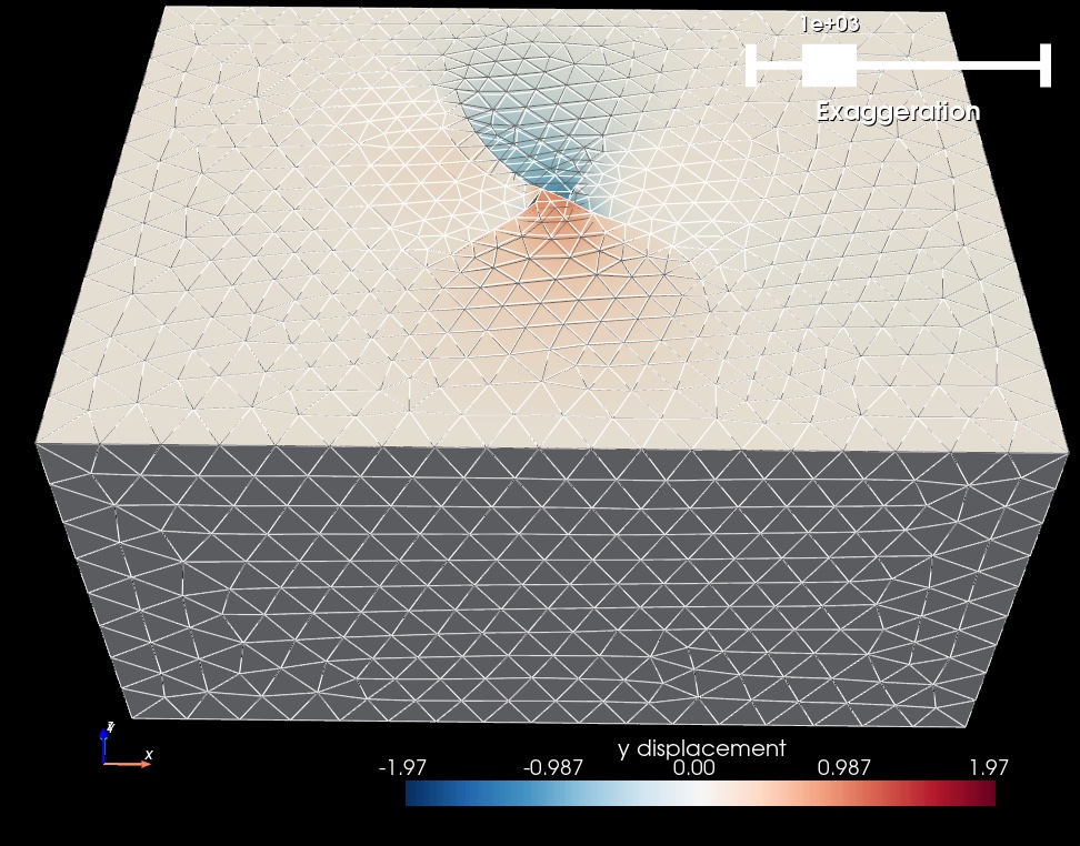
Fig. 127 Solution for Step 2. The colors of the shaded surface indicate the y displacement, and the deformation is exaggerated by a factor of 1000. The undeformed configuration is shown by the gray wireframe. The contrast in material properties across the faults causes the asymmetry in the y displacement field.#