Step 3: Quasistatic Earthquake Cycle

Features

• Triangular cells

• field split preconditioner

• Schur complement

• pylith.meshio.MeshIOPetsc

• pylith.problems.TimeDependent

• pylith.materials.Elasticity

• pylith.materials.IsotropicLinearElasticity

• pylith.meshio.OutputSolnBoundary

• pylith.meshio.DataWriterHDF5

• Quasitatic simulation

• pylith.faults.FaultCohesiveKin

• pylith.bc.DirichletTimeDependent

• spatialdata.spatialdb.SimpleDB

• spatialdata.spatialdb.UniformDB

• pylith.faults.KinSrcConstRate

• pylith.bc.ZeroDB

Simulation parameters

This simulation combines 300 years of interseismic deformation from Step 2 with the coseismic deformation from Step 1 applied at 150 years to create a simple model of an earthquake cycle. Fig. 95 shows the schematic of the boundary conditions. The parameters specific to this example are in step03_eqcycle.cfg.

Fig. 95 Boundary conditions for a simple earthquake cycle with presribed coseismic slip and creep. We combine the coseismic slip from Step 1 with the interseismic slip from Step 2.

On the interface along the top of the subducting oceanic crust and the continental crust and mantle we create two earthquake ruptures. The first rupture applies the coseismic slip from Step 1 at 150 years, while the second rupture prescribes the same steady, aseismic slip as in Step 2. On the interface between the bottom of the subducting oceanic crust and the mantle, we prescribe the same steady, aseismic slip as that in Step 2.

Listing 140 Prescribed slip parameters for Step 3. We only show the details for the top of the slab.

[pylithapp.problem]
interfaces = [fault_slabtop, fault_slabbot]

[pylithapp.problem.interfaces.fault_slabtop]
label = fault_slabtop
label_value = 21
edge = fault_slabtop_edge
edge_value = 31

observers.observer.data_fields = [slip]

eq_ruptures = [creep, earthquake]

# Creep
eq_ruptures.creep = pylith.faults.KinSrcConstRate
eq_ruptures.creep.origin_time = 0.0*year


# Earthquake
eq_ruptures.earthquake = pylith.faults.KinSrcStep
eq_ruptures.earthquake.origin_time = 150.0*year

[pylithapp.timedependent.interfaces.fault_slabtop.eq_ruptures.earthquake]
db_auxiliary_field = spatialdata.spatialdb.SimpleDB
db_auxiliary_field.description = Fault rupture auxiliary field spatial database
db_auxiliary_field.iohandler.filename = fault_coseismic.spatialdb
db_auxiliary_field.query_type = linear

[pylithapp.timedependent.interfaces.fault_slabtop.eq_ruptures.creep]
db_auxiliary_field = spatialdata.spatialdb.SimpleDB
db_auxiliary_field.description = Fault rupture auxiliary field spatial database
db_auxiliary_field.iohandler.filename = fault_slabtop_creep.spatialdb
db_auxiliary_field.query_type = linear

Running the simulation

Listing 141 Run Step 3 simulation

$ pylith step03_eqcycle.cfg

# The output should look something like the following.
 >> /software/unix/py39-venv/pylith-debug/lib/python3.9/site-packages/pylith/meshio/MeshIOObj.py:44:read
 -- meshiopetsc(info)
 -- Reading finite-element mesh
 >> /src/cig/pylith/libsrc/pylith/meshio/MeshIO.cc:94:void pylith::meshio::MeshIO::read(topology::Mesh *)
 -- meshiopetsc(info)
 -- Component 'reader': Domain bounding box:
    (-600000, 600000)
    (-600000, 399.651)

# -- many lines omitted --

61 TS dt 0.05 time 3.
    0 SNES Function norm 5.748198604376e-02 
    Linear solve converged due to CONVERGED_ATOL iterations 178
    1 SNES Function norm 1.127019123456e-11 
  Nonlinear solve converged due to CONVERGED_FNORM_ABS iterations 1
62 TS dt 0.05 time 3.05
 >> /software/unix/py39-venv/pylith-debug/lib/python3.9/site-packages/pylith/problems/Problem.py:201:finalize
 -- timedependent(info)
 -- Finalizing problem.

The beginning of the output written to the terminal is identical to that from Steps 1 and 2. At the end of the output, we see that the simulation advanced the solution 62 time steps. Remember that the PETSc TS monitor shows the nondimensionalized time and time step values.

Visualizing the results

In Fig. 96 we use ParaView to visualize the x displacement field using the viz/plot_dispwarp.py Python script. First, we start ParaView from the examples/subduction-2d directory. Next, we override the default name of the simulation file with the name of the current simulation.

Listing 142 Set the simulation in the ParaView Python Shell.

>>> SIM = "step03_eqcycle"

Finally, we run the viz/plot_dispwarp.py Python script as described in ParaView Python Scripts.

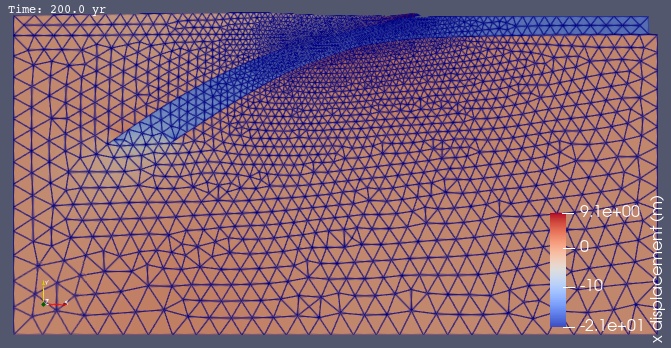
Fig. 96 Solution for Step 3 at t=200 yr. The colors of the shaded surface indicate the magnitude of the x displacement, and the deformation is exaggerated by a factor of 1000.