Step 1: Static Coseismic Slip#
This example involves a static simulation that solves for the deformation from prescribed coseismic slip on the subduction interface. The depth variation in the prescribed slip is based on the 2011 Tohoku-oki earthquake. Fig. 90 shows the boundary conditions on the domain.

Fig. 90 Boundary conditions for static coseismic slip on the subduction interface. We prescribe reverse slip that varies with depth and roller boundary conditions on the lateral sides and bottom of the domain.#
Features
Triangular cells
field split preconditioner
Schur complement
pylith.meshio.MeshIOPetsc
pylith.problems.TimeDependent
pylith.materials.Elasticity
pylith.materials.IsotropicLinearElasticity
pylith.meshio.OutputSolnBoundary
pylith.meshio.DataWriterHDF5
Static simulation
pylith.faults.FaultCohesiveKin
pylith.bc.DirichletTimeDependent
spatialdata.spatialdb.SimpleDB
pylith.faults.KinSrcStep
pylith.bc.ZeroDB
Simulation parameters#
The parameters specific to this example are in step01_coseismic.cfg and include:
pylithapp.metadataMetadata for this simulation. Even when the author and version are the same for all simulations in a directory, we prefer to keep that metadata in each simulation file as a reminder to keep it up-to-date for each simulation.pylithappParameters defining where to write the output.pylithapp.problemParameters for the solution field with displacement and Lagrange multiplier subfields.pylithapp.problem.faultParameters for prescribed slip on the fault.
Important
In 2D simulations slip is specified in terms of opening and left-lateral components. This provides a consistent, unique sense of slip that is independent of the fault orientation. For our geometry in this example, right-lateral slip corresponds to reverse slip on the subduction interface.
$ pylith step01_coseismic.cfg

# The output should look something like the following.
 >> /software/unix/py39-venv/pylith-debug/lib/python3.9/site-packages/pylith/meshio/MeshIOObj.py:44:read
 -- meshiopetsc(info)
 -- Reading finite-element mesh
 >> /src/cig/pylith/libsrc/pylith/meshio/MeshIO.cc:94:void pylith::meshio::MeshIO::read(topology::Mesh *)
 -- meshiopetsc(info)
 -- Component 'reader': Domain bounding box:
    (-600000, 600000)
    (-600000, 399.651)
 >> /software/unix/py39-venv/pylith-debug/lib/python3.9/site-packages/pylith/problems/Problem.py:116:preinitialize
 -- timedependent(info)
 -- Performing minimal initialization before verifying configuration.
 >> /software/unix/py39-venv/pylith-debug/lib/python3.9/site-packages/pylith/problems/Solution.py:44:preinitialize
 -- solution(info)
 -- Performing minimal initialization of solution.
 >> /software/unix/py39-venv/pylith-debug/lib/python3.9/site-packages/pylith/problems/Problem.py:175:verifyConfiguration
 -- timedependent(info)
 -- Verifying compatibility of problem configuration.
 >> /software/unix/py39-venv/pylith-debug/lib/python3.9/site-packages/pylith/problems/Problem.py:221:_printInfo
 -- timedependent(info)
 -- Scales for nondimensionalization:
    Length scale: 1000*m
    Time scale: 3.15576e+09*s
    Pressure scale: 3e+10*m**-1*kg*s**-2
    Density scale: 2.98765e+23*m**-3*kg
    Temperature scale: 1*K
 >> /software/unix/py39-venv/pylith-debug/lib/python3.9/site-packages/pylith/problems/Problem.py:186:initialize
 -- timedependent(info)
 -- Initializing timedependent problem with quasistatic formulation.
 >> /src/cig/pylith/libsrc/pylith/utils/PetscOptions.cc:235:static void pylith::utils::_PetscOptions::write(pythia::journal::info_t &, const char *, const pylith::utils::PetscOptions &)
 -- petscoptions(info)
 -- Setting PETSc options:
fieldsplit_displacement_ksp_type = preonly
fieldsplit_displacement_pc_type = lu
fieldsplit_lagrange_multiplier_fault_ksp_type = preonly
fieldsplit_lagrange_multiplier_fault_pc_type = lu
ksp_atol = 1.0e-12
ksp_converged_reason = true
ksp_error_if_not_converged = true
ksp_rtol = 1.0e-12
pc_fieldsplit_schur_factorization_type = lower
pc_fieldsplit_schur_precondition = selfp
pc_fieldsplit_schur_scale = 1.0
pc_fieldsplit_type = schur
pc_type = fieldsplit
pc_use_amat = true
snes_atol = 1.0e-9
snes_converged_reason = true
snes_error_if_not_converged = true
snes_monitor = true
snes_rtol = 1.0e-12
ts_error_if_step_fails = true
ts_monitor = true
ts_type = beuler

 >> /software/unix/py39-venv/pylith-debug/lib/python3.9/site-packages/pylith/problems/TimeDependent.py:139:run
 -- timedependent(info)
 -- Solving problem.
0 TS dt 0.05 time -0.05
    0 SNES Function norm 5.454651006059e-01
    Linear solve converged due to CONVERGED_ATOL iterations 85
    1 SNES Function norm 3.437540896787e-12
  Nonlinear solve converged due to CONVERGED_FNORM_ABS iterations 1
1 TS dt 0.05 time 0.
 >> /software/unix/py39-venv/pylith-debug/lib/python3.9/site-packages/pylith/problems/Problem.py:201:finalize
 -- timedependent(info)
 -- Finalizing problem.
At the beginning of the output written to the terminal, we see that PyLith is reading the mesh using the MeshIOPetsc reader and that it found the domain to extend from -600 km to +600 km in the x direction and from -600 km to 0 in the y direction.
The output also includes the scales used for nondimensionalization and the default PETSc options.
At the end of the output written to the termial, we see that the solver advanced the solution one time step (static simulation).
The linear solve converged after 85 iterations and the norm of the residual met the absolute convergence tolerance (ksp_atol) .
The nonlinear solve converged in 1 iteration, which we expect because this is a linear problem, and the residual met the absolute convergence tolerance (snes_atol).
Visualizing the results#
The output directory contains the simulation output.
Each “observer” writes its own set of files, so the solution over the domain is in one set of files, the boundary condition information is in another set of files, and the material information is in yet another set of files.
The HDF5 (.h5) files contain the mesh geometry and topology information along with the solution fields.
The Xdmf (.xmf) files contain metadata that allow visualization tools like ParaView to know where to find the information in the HDF5 files.
To visualize the data using ParaView or Visit, load the Xdmf files.
In Fig. 91 we use ParaView to visualize the x displacement field using the viz/plot_dispwarp.py Python script.
We start ParaView from the examples/subduction-2d directory and then run the viz/plot_dispwarp.py Python script as described in ParaView Python Scripts.
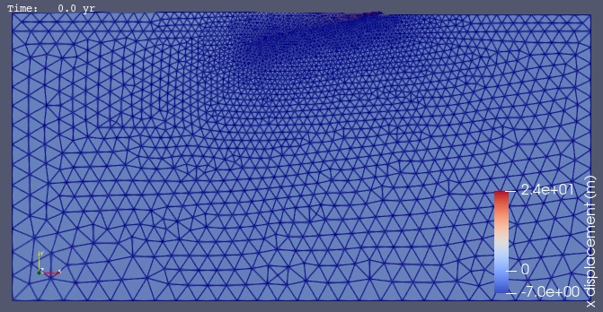
Fig. 91 Solution for Step 1. The colors of the shaded surface indicate the magnitude of the x displacement, and the deformation is exaggerated by a factor of 1000.#