Step 4: Variable Coseismic Slip#
We use this example to illustrate prescribing slip that varies along the strike of the fault. This example also serves as a means to generate coseismic displacements at fake GPS stations. In Step 6 we will use the displacements at these stations along with static Green’s functions computed in Step 5 to invert for the slip on the fault.
We prescribe left-lateral slip that varies along the strike of the fault with fixed displacements on the +x and -x boundaries (Fig. 60), similar to what we had in Step 1. The slip is nonzero over the region -20 km \(\le\) y \(\le\) +20 km with a peak slip of 80 cm at y=-0.5 km (Fig. 61).
This example involves a static simulation that solves for the deformation from prescribed coseismic slip on the fault. We specify 2 meters of right-lateral slip. Fig. 60 shows the boundary conditions on the domain.

Fig. 60 Boundary conditions for static coseismic slip. We set the x and y displacement to zero on the +x and -x boundaries and prescribe left-lateral slip that varies along strike.#

Fig. 61 Prescribed left-lateral slip that varies along the strike of the fault. A strike of 0 corresponds to y=9.#
Features
Triangular cells
pylith.meshio.MeshIOPetsc
pylith.problems.TimeDependent
pylith.materials.Elasticity
pylith.materials.IsotropicLinearElasticity
pylith.faults.FaultCohesiveKin
pylith.faults.KinSrcStep
field split preconditioner
Schur complement preconditioner
pylith.bc.DirichletTimeDependent
spatialdata.spatialdb.UniformDB
pylith.meshio.OutputSolnBoundary
pylith.meshio.DataWriterHDF5
Static simulation
Simulation parameters#
The parameters specific to this example are in step04_varslip.cfg.
These include:
pylithapp.metadataMetadata for this simulation. Even when the author and version are the same for all simulations in a directory, we prefer to keep that metadata in each simulation file as a reminder to keep it up-to-date for each simulation.pylithappParameters defining where to write the output.pylithapp.problemParameters for the solution field and output.pylithapp.problem.faultParameters for prescribed slip on the fault.
We increase the basis order of the solution subfields to 2 to better resolve the spatial variation in slip.
We also add output of the solution at fake GPS stations given in the file gps_stations.txt.
You can use the Python script generate_gpsstations.py to generate a different random set of stations; the default parameters will generate the provided gps_stations.txt file.
$ pylith step04_varslip.cfg

# The output should look something like the following.
 >> /software/unix/py39-venv/pylith-debug/lib/python3.9/site-packages/pylith/meshio/MeshIOObj.py:44:read
 -- meshiopetsc(info)
 -- Reading finite-element mesh
 >> /src/cig/pylith/libsrc/pylith/meshio/MeshIO.cc:94:void pylith::meshio::MeshIO::read(topology::Mesh *)
 -- meshiopetsc(info)
 -- Component 'reader': Domain bounding box:
    (-50000, 50000)
    (-75000, 75000)

# -- many lines omitted --

 >> /software/unix/py39-venv/pylith-debug/lib/python3.9/site-packages/pylith/problems/TimeDependent.py:139:run
 -- timedependent(info)
 -- Solving problem.
0 TS dt 0.01 time 0.
    0 SNES Function norm 3.840123479624e-03
    Linear solve converged due to CONVERGED_ATOL iterations 73
    1 SNES Function norm 2.286140232631e-12
  Nonlinear solve converged due to CONVERGED_FNORM_ABS iterations 1
1 TS dt 0.01 time 0.01
 >> /software/unix/py39-venv/pylith-debug/lib/python3.9/site-packages/pylith/problems/Problem.py:201:finalize
 -- timedependent(info)
 -- Finalizing problem.
The beginning of the output written to the terminal matches that in our previous simulations.
At the end of the output written to the termial, we see that the solver advanced the solution one time step (static simulation).
The linear solve converged after 73 iterations and the norm of the residual met the absolute convergence tolerance (ksp_atol).
The nonlinear solve converged in 1 iteration, which we expect because this is a linear problem, and the residual met the absolute convergence tolerance (snes_atol).
Visualizing the results#
The output directory contains the simulation output.
Each “observer” writes its own set of files, so the solution over the domain is in one set of files, the boundary condition information is in another set of files, and the material information is in yet another set of files.
The HDF5 (.h5) files contain the mesh geometry and topology information along with the solution fields.
The Xdmf (.xmf) files contain metadata that allow visualization tools like ParaView to know where to find the information in the HDF5 files.
To visualize the data using ParaView or Visit, load the Xdmf files.
In Fig. 62 we use ParaView to visualize the y displacement field using the viz/plot_dispwarp.py Python script.
As in Steps 2-3 we override the default name of the simulation file with the name of the current simulation.
>>> SIM = "step04_varslip"
Next we run the viz/plot_dispwarp.py Python script as described in ParaView Python Scripts.
We can add the displacement vectors at the fake GPS stations using the viz/plot_dispstations.py Python script.
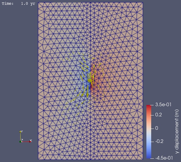
Fig. 62 Solution for Step 4. The colors of the shaded surface indicate the magnitude of the y displacement, and the deformation is exaggerated by a factor of 1000. The displacement vectors at the fake GPS stations use en exaggeration factor of 50,000.#