Step 1: Axial Extension#
This example corresponds to axial extension in the x direction.
We apply Dirichlet (displacement) boundary conditions for the x displacement on the +x (boundary_xpos) and -x (boundary_xneg) boundaries.
We apply roller Dirichlet boundary conditions on the -y (boundary_yneg) boundary.
Fig. 26 shows the boundary conditions on the domain.

Fig. 26 Boundary conditions for axial extension in the x-direction. We constrain the x displacement on the +x and -x boundaries and set the y displacement to zero on the -y boundary.#
Features
Quadrilateral cells
pylith.meshio.MeshIOAscii
pylith.problems.TimeDependent
pylith.materials.Elasticity
pylith.materials.IsotropicLinearElasticity
spatialdata.spatialdb.UniformDB
pylith.meshio.DataWriterHDF5
Static simulation
ILU preconditioner
pylith.bc.DirichletTimeDependent
spatialdata.spatialdb.ZeroDB
Simulation parameters#
The parameters specific to this example are in step01_axialdisp.cfg.
These include:
pylithapp.metadataMetadata for this simulation. Even when the author and version are the same for all simulations in a directory, we prefer to keep that metadata in each simulation file as a reminder to keep it up-to-date for each simulation.pylithappParameters defining where to write the output.pylithapp.problem.solutionSpecify the basis order for the solution fields, in this case thedisplacementfield.pylithapp.problem.bcParameters for the boundary conditions.
$ pylith step01_axialdisp.cfg

# The output should look something like the following.
 >> /software/unix/py39-venv/pylith-debug/lib/python3.9/site-packages/pylith/meshio/MeshIOObj.py:44:read
 -- meshioascii(info)
 -- Reading finite-element mesh
 >> /src/cig/pylith/libsrc/pylith/meshio/MeshIO.cc:94:void pylith::meshio::MeshIO::read(topology::Mesh *)
 -- meshioascii(info)
 -- Component 'reader': Domain bounding box:
    (-6000, 6000)
    (-16000, -0)
 >> /software/unix/py39-venv/pylith-debug/lib/python3.9/site-packages/pylith/problems/Problem.py:116:preinitialize
 -- timedependent(info)
 -- Performing minimal initialization before verifying configuration.
 >> /software/unix/py39-venv/pylith-debug/lib/python3.9/site-packages/pylith/problems/Solution.py:44:preinitialize
 -- solution(info)
 -- Performing minimal initialization of solution.
 >> /software/unix/py39-venv/pylith-debug/lib/python3.9/site-packages/pylith/problems/Problem.py:175:verifyConfiguration
 -- timedependent(info)
 -- Verifying compatibility of problem configuration.
 >> /software/unix/py39-venv/pylith-debug/lib/python3.9/site-packages/pylith/problems/Problem.py:221:_printInfo
 -- timedependent(info)
 -- Scales for nondimensionalization:
    Length scale: 1000*m
    Time scale: 3.15576e+09*s
    Pressure scale: 3e+10*m**-1*kg*s**-2
    Density scale: 2.98765e+23*m**-3*kg
    Temperature scale: 1*K
 >> /software/unix/py39-venv/pylith-debug/lib/python3.9/site-packages/pylith/problems/Problem.py:186:initialize
 -- timedependent(info)
 -- Initializing timedependent problem with quasistatic formulation.
 >> /src/cig/pylith/libsrc/pylith/utils/PetscOptions.cc:235:static void pylith::utils::_PetscOptions::write(pythia::journal::info_t &, const char *, const pylith::utils::PetscOptions &)
 -- petscoptions(info)
 -- Setting PETSc options:
ksp_atol = 1.0e-12
ksp_converged_reason = true
ksp_error_if_not_converged = true
ksp_rtol = 1.0e-12
pc_type = lu
snes_atol = 1.0e-9
snes_converged_reason = true
snes_error_if_not_converged = true
snes_monitor = true
snes_rtol = 1.0e-12
ts_error_if_step_fails = true
ts_monitor = true
ts_type = beuler

 >> /software/unix/py39-venv/pylith-debug/lib/python3.9/site-packages/pylith/problems/TimeDependent.py:139:run
 -- timedependent(info)
 -- Solving problem.
0 TS dt 0.01 time 0.
    0 SNES Function norm 1.245882095312e-02
    Linear solve converged due to CONVERGED_ATOL iterations 1
    1 SNES Function norm 6.738354969624e-18
  Nonlinear solve converged due to CONVERGED_FNORM_ABS iterations 1
1 TS dt 0.01 time 0.01
 >> /software/unix/py39-venv/pylith-debug/lib/python3.9/site-packages/pylith/problems/Problem.py:201:finalize
 -- timedependent(info)
 -- Finalizing problem.
At the beginning of the output written to the terminal, we see that PyLith is reading the mesh using the MeshIOAscii reader and that it found the domain to extend from -6000 m to +6000 m in the x direction and from -16000 m to 0 m in the y direction.
We also see the scales used to nondimensionalize the problem.
The density scale is very large for quasistatic problems.
Near the end of the output written to the terminal, we see the PETSc options PyLith selected based on the governing equations and formulation as discussed in PETSc Options.
The solver advanced the solution one time step (static simulation).
The linear solve converged in 1 iteration, consistent with the LU preconditioner.
The norm of the residual met the absolute tolerance convergence criterion (ksp_atol).
The nonlinear solve converged in 1 iteration, which we expect because this is a linear problem, and the residual met the absolute convergence tolerance (snes_atol).
Visualizing the results#
The output directory contains the simulation output.
Each “observer” writes its own set of files, so the solution over the domain is in one set of files, the boundary condition information is in another set of files, and the material information is in yet another set of files.
The HDF5 (.h5) files contain the mesh geometry and topology information along with the solution fields.
The Xdmf (.xmf) files contain metadata that allow visualization tools like ParaView to know where to find the information in the HDF5 files.
To visualize the data using ParaView or Visit, load the Xdmf files.
In Fig. 27 we use ParaView to visualize the x displacement field using the viz/plot_dispwarp.py Python script.
First, we first start ParaView from the examples/box-2d directory.
$ PATH_TO_PARAVIEW/paraview

# For macOS, it will be something like
$ /Applications/ParaView-5.10.1.app/Contents/MacOS/paraview
Next we run the viz/plot_dispwarp.py Python script as described in ParaView Python Scripts.
For Step 1 we do not need to change any of the default values.
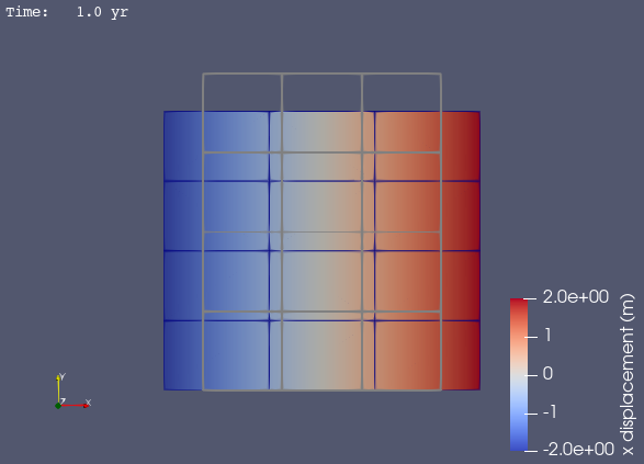
Fig. 27 Solution for Step 1. The colors of the shaded surface indicate the magnitude of the x displacement, and the deformation is exaggerated by a factor of 1000. The undeformed configuration is show by the gray wireframe.#